Download
1 / 33
780 likes | 1.71k Vues
Series AC Circuits Analysis. ET 242 Circuit Analysis II. E lectrical and T elecommunication Engineering Technology Professor Jang. Acknowledgement.

E N D
Series AC Circuits Analysis ET 242 Circuit Analysis II Electrical and Telecommunication Engineering Technology Professor Jang
Acknowledgement I want to express my gratitude to Prentice Hall giving me the permission to use instructor’s material for developing this module. I would like to thank the Department of Electrical and Telecommunications Engineering Technology of NYCCT for giving me support to commence and complete this module. I hope this module is helpful to enhance our students’ academic performance.
OUTLINES • Introduction to Series ac Circuits Analysis • Impedance and Phase Diagram • Series Configuration • Voltage Divider Rule • Frequency Response for Series ac Circuits Key Words: Impedance, Phase, Series Configuration, Voltage Divider Rule ET 242 Circuit Analysis II – Sinusoidal Alternating Waveforms Boylestad2
Series & Parallel ac Circuits Phasor algebra is used to develop a quick, direct method for solving both series and parallel ac circuits. The close relationship that exists between this method for solving for unknown quantities and the approach used for dc circuits will become apparent after a few simple examples are considered. Once this association is established, many of the rules (current divider rule, voltage divider rule, and so on) for dc circuits can be applied to ac circuits. Series ac Circuits Impedance & the Phasor Diagram – Resistive Elements From previous lesson we found, for the purely resistive circuit in Fig. 15-1, that v and i were in phase, and the magnitude Figure 15.1 Resistive ac circuit. ET 242 Circuit Analysis II – Sinusoidal Alternating Waveforms Boylestad3
Ex. 15-1 Using complex algebra, find the current i for the circuit in Fig. 15-2. Sketch the waveforms of v and i. FIGURE 15.2 FIGURE 15.3 ET 242 Circuit Analysis II – Sinusoidal Alternating Waveforms Boylestad5
Ex. 15-2 Using complex algebra, find the voltage v for the circuit in Fig. 15- 4. Sketch the waveforms of v and i. FIGURE 15.4 FIGURE 15.5 ET 242 Circuit Analysis II – Sinusoidal Alternating Waveforms Boylestad6
Series ac Circuits Impedance & the Phasor Diagram – Inductive Elements From previous lesson we found that the purely inductive circuit in Fig. 15-7, voltage leads the current by 90° and that the reactance of the coil XL is determined by ωL. Figure 15.7Inductive ac circuit. Since v leads i by 90°, i must have an angle of – 90° associated with it. To satisfy this condition, θL must equal + 90°. Substituting θL = 90°, we obtain We use the fact that θL = 90° in the following polar format for inductive reactance to ensure the proper phase relationship between the voltage and current of an inductor: ET 242 Circuit Analysis II – Sinusoidal Alternating Waveforms Boylestad3
Ex. 15-3 Using complex algebra, find the current i for the circuit in Fig. 15- 8. Sketch the v and i curves. FIGURE 15.9 FIGURE 15.8 ET 242 Circuit Analysis II – Sinusoidal Alternating Waveforms Boylestad5
Ex. 15-4 Using complex algebra, find the voltage v for the circuit in Fig. 15- 10. Sketch the v and i curves. FIGURE 15.10 FIGURE 15.11 ET 242 Circuit Analysis II – Sinusoidal Alternating Waveforms Boylestad9
Ex. 13-3 Determine the frequency of the waveform in Fig. 13-9. From the figure, T = (25 ms – 5 ms) or (35 ms – 15 ms) = 20 ms, and FIGURE 13.9 ET 242 Circuit Analysis II – Sinusoidal Alternating Waveforms Boylestad10
The Sinusoidal Waveform Consider the power of the following statement: The sinusoidal waveform is the only alternating waveform whose shape is unaffected by the response characteristics of R, L, and C element. In other word, if the voltage or current across a resistor, inductor, or capacitor is sinusoidal in nature, the resulting current or voltage for each will also have sinusoidal characteristics, as shown in Fig. 13-12. FIGURE 13.12The sine wave is the only alternating waveform whose shape is not altered by the response characteristics of a pure resistor, indicator, or capacitor. ET162 Circuit Analysis – Ohm’s Law Boylestad11
The unit of measurement for the horizontal axis can be time, degree, or radians. The term radian can be defined as follow: If we mark off a portion of the circumference of a circle by a length equal to the radius of the circle, as shown in Fig. 13-13, the angle resulting is called 1 radian. The result is One full circle has 2π radians, as shown in Fig. 13-14. That is 2π rad = 360° 2π = 2(3.142) = 6.28 2π(57.3°) = 6.28(57.3°) = 359.84° ≈ 360° FIGURE 13.13Defining the radian. 1 rad = 57.296° ≈ 57.3° where 57.3° is the usual approximation applied. ET 242 Circuit Analysis II – Sinusoidal Alternating Waveforms Boylestad2 FIGURE 13.14There are 2π radian in one full circle of 360°.
A number of electrical formulas contain a multiplier of π. For this reason, it is sometimes preferable to measure angles in radians rather than in degrees. The quantity is the ratio of the circumference of a circle to its diameter. For comparison purposes, two sinusoidal voltages are in Fig. 13-15 using degrees and radians as the units of measurement for the horizontal axis. FIGURE 13.15Plotting a sine wave versus (a) degrees and (b) radians. ET 242 Circuit Analysis – Sinusoidal Alternating Waveforms Boylestad13
In Fig. 13-16, the time required to complete one revolution is equal to the period (T) of the sinusoidal waveform. The radians subtended in this time interval are 2π. Substituting, we have ω = 2π/T or 2πf (rad/s) FIGURE 13.17Demonstrating the effect of ω on the frequency and period FIGURE 13.16Generating a sinusoidal waveform through the vertical projection of a rotating vector. ET 242 Circuit Analysis – Sinusoidal Alternating Waveforms Boylestad14
Ex. 13-4 Determine the angular velocity of a sine wave having a frequency of 60 Hz. ω = 2πf = (2π)(60 Hz) ≈ 377 rad/s Ex. 13-5 Determine the frequency and period of the sine wave in Fig. 13-17 (b). ET 242 Circuit Analysis II – Sinusoidal Alternating Waveforms Boylestad15
Ex. 13-6 Given ω = 200 rad/s, determine how long it will take the sinusoidal waveform to pass through an angle of 90°. α = ωt, and t = α / ω Ex. 13-7 Find the angle through which a sinusoidal waveform of 60 Hz will pass in a period of 5 ms. α = ωt, or α = 2πft = (2π)(60 Hz)(5 × 10⁻³ s) = 1.885 rad ET 242 Circuit Analysis II – Sinusoidal Alternating Waveforms Boylestad16
General Format for the Sinusoidal Voltage or Current The basic mathematical format for the sinusoidal waveform is Am sin α = Am sin ωt where Am is the peak value of the waveform and α is the unit of measure for the horizontal axis, as shown in Fig. 13-18. For electrical quantities such as current and voltage, the general format is i = Im sin ωt = Im sin α e = Em sin ωt = Em sin α where the capital letters with the subscript m represent the amplitude, and the lowercase letters I and e represent the instantaneous value of current and voltage at any time t. FIGURE 13.18Basic sinusoidal function. ET 242 Circuit Analysis II – Sinusoidal Alternating Waveforms Boylestad17
Ex. 13-8 Given e = 5 sin α, determine e at α = 40° and α = 0.8π. Ex. 13-11 Given i = 6×10⁻³ sin 100t, determine i at t = 2 ms. ET 242 Circuit Analysis II – Sinusoidal Alternating Waveforms Boylestad18
Phase Relations If the waveform is shifted to the right or left of 0°, the expression becomes Am sin (ωt± θ) where θ is the angle in degrees or radiations that the waveform has been shifted. If the waveform passes through the horizontal axis with a positive going slope before 0°, as shown in Fig. 13-27, the expression is Am sin (ωt+ θ) If the waveform passes through the horizontal axis with a positive going slope after 0°, as shown in Fig. 13-28, the expression is Am sin (ωt– θ) FIGURE 13.27Defining the phase shift for a sinusoidal function that crosses the horizontal axis with a positive slope before 0°. FIGURE 13.28Defining the phase shift for a sinusoidal function that crosses the horizontal axis with a positive slope after 0°.
If the waveform crosses the horizontal axis with a positive-going slope 90° (π/2) sooner, as shown in Fig. 13-29, it is called a cosine wave; that is sin (ωt + 90°)=sin (ωt + π/2) = cos πt or sin ωt = cos (ωt – 90°) = cos (ωt – π/2) FIGURE 13.29Phase relationship between a sine wave and a cosine wave. cos α = sin (α + 90°) sin α = cos (α – 90°) – sin α = sin (α ± 180°) – cos α = sin (α + 270°) = sin (α – 90°) sin (–α) = –sin α cos (–α) = cos α ET 242 Circuit Analysis II – Sinusoidal Alternating Waveforms Boylestad20
The oscilloscope is an instrument that will display the sinusoidal alternating waveform in a way that permit the reviewing of all of the waveform’s characteristics. The vertical scale is set to display voltage levels, whereas the horizontal scale is always in units of time. Phase Relations – The Oscilloscope Ex. 13-13 Find the period, frequency, and peak value of the sinusoidal waveform appearing on the screen of the oscilloscope in Fig. 13-36. Note the sensitivities provided in the figure. FIGURE 13.36 ET 242 Circuit Analysis II – Sinusoidal Alternating Waveforms Boylestad21
An oscilloscope can also be used to make phase measurements between two sinusoidal waveforms. Oscilloscopes have the dual-trace option, that is, the ability to show two waveforms at the same time. It is important that both waveforms must have the same frequency. The equation for the phase angle can be introduced using Fig. 13-37. First, note that each sinusoidal function has the same frequency, permitting the use of either waveform to determine the period. For the waveform chosen in Fig. 13-37, the period encompasses 5 divisions at 0.2 ms/div. The phase shift between the waveforms is 2 divisions. Since the full period represents a cycle of 360°, the following ratio can be formed: FIGURE 13.37Finding the phase angle between waveforms using a dual-trace oscilloscope. ET 242 Circuit Analysis II – Sinusoidal Alternating Waveforms Boylestad 22
Average Value The concept of the average value is an important one in most technical fields. In Fig. 13-38(a), the average height of the sand may be required to determine the volume of sand available. The average height of the sand is that height obtained if the distance from one end to the other is maintained while the sand is leveled off, as shown in Fig. 13-38(b). The area under the mound in Fig. 13-38(a) then equals the area under the rectangular shape in Fig. 13-38(b) as determined by A = b × h. FIGURE 13.38Defining average value. FIGURE 13.39Effect of distance (length) on average value. FIGURE 13.40Effect of depressions (negative excursions) on average value.
Ex. 13-14 Determine the average value of the waveforms in Fig.13-42. FIGURE 13.42 • By inspection, the area above the axis equals the area below over one cycle, resulting in an average value of zero volts. ET 242 Circuit Analysis II – Sinusoidal Alternating Waveforms Boylestad24
Ex. 13-15 Determine the average value of the waveforms over one full cycle: a. Fig. 13-44. b. Fig. 13-45 FIGURE 13.44 FIGURE 13.45 ET 242 Circuit Analysis II – Sinusoidal Alternating Waveforms Boylestad25
Ex. 13-16 Determine the average value of the sinusoidal waveforms in Fig. 13-51. The average value of a pure sinusoidal waveform over one full cycle is zero. FIGURE 13.51 Ex. 13-17 Determine the average value of the waveforms in Fig. 13-52. Results in an average or dc level of – 7 mV, as noted by the dashed line in Fig. 13-52. FIGURE 13.52 ET 242 Circuit Analysis II – Sinusoidal Alternating Waveforms Boylestad26
Effective (rms) Values This section begins to relate dc and ac quantities with respect to the power delivered to a load. The average power delivered by the ac source is just the first term, since the average value of a cosine wave is zero even though the wave may have twice the frequency of the original input current waveform. Equation the average power delivered by the ac generator to that delivered by the dc source, Which, in words, states that The equivalent dc value of a sinusoidal current or voltage is 1 / √2 or 0.707 of its peak value. The equivalent dc value is called the rms or effective value of the sinusoidal quantity. Similarly, ET 242 Circuit Analysis II – Sinusoidal Alternating Waveforms Boylestad27
Ex. 13-20 Find the rms values of the sinusoidal waveform in each part of Fig. 13-58. FIGURE 13.58 • b. Irms = 8.48 mA • Note that frequency did not change the • effective value in (b) compared to (a). ET 242 Circuit Analysis II – Sinusoidal Alternating Waveforms Boylestad28
Ex. 13-21 The 120 V dc source in Fig. 13-59(a) delivers 3.6 W to the load. Determine the peak value of the applied voltage (Em) and the current (Im) if the ac source [Fig. 13-59(b)] is to deliver the same power to the load. FIGURE 13.59 ET 242 Circuit Analysis II – Sinusoidal Alternating Waveforms Boylestad29
Ex. 13-22 Find the rms value of the waveform in Fig. 13-60. FIGURE 13.61 FIGURE 13.60 Ex. 13-24 Determine the average and rms values of the square wave in Fig. 13-64. By inspection, the average value is zero. FIGURE 13.64 ET 242 Circuit Analysis II – Sinusoidal Alternating Waveforms Boylestad30
Ac Meters and Instruments It is important to note whether the DMM in use is a true rms meter or simply meter where the average value is calculated to indicate the rms level. A true rms meter reads the effective value of any waveform and is not limited to only sinusoidal waveforms. Fundamentally, conduction is permitted through the diodes in such a manner as to convert the sinusoidal input of Fig. 13-68(a) to one having been effectively “flipped over” by the bridge configuration. The resulting waveform in Fig. 13-68(b) is called a full-wave rectified waveform. FIGURE 13.68(a) Sinusoidal input; (b) full-wave rectified signal. ET 242 Circuit Analysis II – Sinusoidal Alternating Waveforms Boylestad31
Forming the ratio between the rms and dc levels results in Meter indication = 1.11 (dc or average value) Full-wave Ex. 13-25 Determine the reading of each meter for each situation in Fig. 13-71(a) &(b). For Fig. 13-71(a), situation (1): Meter indication = 1.11(20V) = 22.2V For Fig.13-71(a), situation (2): Vrms = 0.707Vm = 0.707(20V) = 14.14V For Fig. 13-71(b), situation (1): Vrms = Vdc = 25 V For Fig.13-71(b), situation (2): Vrms = 0.707Vm = 0.707(15V) ≈ 10.6V FIGURE 13.71 ET 242 Circuit Analysis II – Sinusoidal Alternating Waveforms Boylestad2