Advancements in CO2 Flux Estimation: 4-D Variational Data Assimilation Techniques
This presentation discusses the use of 4-D Variational (4-D Var) data assimilation techniques to estimate carbon dioxide (CO2) sources and sinks at fine spatial and temporal scales. The focus is on the mathematical foundations, methodological advantages, and recent results derived from using these techniques. It highlights the comparison between variational methods and ensemble filters, emphasizing the benefits of a two-sided smoother for accurate flux and concentration estimates. Future prospects include enhancing predictive capabilities by integrating remotely-sensed data and improving spatial resolution.

Advancements in CO2 Flux Estimation: 4-D Variational Data Assimilation Techniques
E N D
Presentation Transcript
Carbon Cycle Data Assimilation with a Variational Approach (“4-D Var”) David Baker CGD/TSS with Scott Doney, Dave Schimel, Britt Stephens, and Roger Dargaville 24 Sept 2004
Outline • The problem: estimate CO2 sources and sinks at fine space/time scales (2° x 2.5°, hourly/daily) • Method: • Why use 4-D Var? (Kalman) filtering, smoothing, and variational methods – pros and cons • Mathematical background of 4-D Var applied to atmospheric trace gases • Some 4-D Var results using simulated truth • Additional topics to ponder: • 100 descent iterations 100 ensemble members? • Error estimates: 4-D Var vs. ensemble filters
Transport: surface fluxes concentrations 0 H fluxes Transport basis functions concentrations
Present Future Shift towards newer instruments/platforms: • More continuous analyzers, new cheap in situ analyzers • Aircraft, towers (flux & tall), ships/planes of opportunity • CO2-sondes, tethered balloons, etc. • Satellite-based column-integrated CO2, maybe CO2 profiles Higher frequency with better spatial coverage -- will permit more detail to be estimated More sensitive to continental air, detailed flow features -- synoptic meteorology, diurnal cycle must be resolved Solve for the fluxes at the resolution of the transport model • 2° x 2.5°, 25 levels, daily/hourly time step • With current inversion techniques, computations grow as O(N3)… more efficient techniques required (iterative vs. direct inversions, adjoint allows efficient gradient computation, minimal storage)
For retrospective analyses, a 2-sided smoother gives more accurate estimates than a 1-sided filter. The 4-D Var method is 2-sided, like a smoother. (Gelb, 1974)
Variational Data Assimilation vs. Ensemble (Kalman) filter Pros: • Greater accuracy achieved with 2-sided smoother than 1-sided filter • Initial transients reduced Cons: • Adjoint model required • [Correlations are pre-specified, rather than calculated, as with a Kalman filter]
4-D Var Data Assimilation Method • Find optimal fluxes u and initial CO2 field xo to minimize • subject to the dynamical constraint • where • x are state variables (CO2 concentrations), • v are independent variables used in model but not optimized, • z are the observations, • R is the covariance matrix for z, • uo is an a priori estimate of the fluxes, • Puo is the covariance matrix for uo, • xo is an a priori estimate of the initial concentrations, • Pxo is the covariance matrix for xo
4-D Var Data Assimilation Method Adjoin the dynamical constraints to the cost function using Lagrange multipliers SettingF/xi = 0 gives an equation for i, the adjoint of xi: The adjoints to the control variables are given byF/uiandF/xooas: The optimal u and xo may then be found iteratively by
4-D Var Iterative Optimization Procedure 0 x0 ° Forward Transport Forward Transport Estimated Fluxes “True” Fluxes 1 2 Modeled Concentrations “True” Concentrations ° x1 ° Measurement Sampling Measurement Sampling x2 Modeled Measurements “True” Measurements Assumed Measurement Errors D/(Error)2 3 x3 ° Weighted Measurement Residuals Flux Update Adjoint Transport Adjoint Fluxes = Minimum of cost function J
Prior Truth OSSE fluxes, snapshot for Jan 1st Estimate (30 descent steps)
Prior - Truth Estimate - Truth
Future Plans for CO2 • Assimilate remotely-sensed data • Finer resolution (1º x 1º, or regional) • Improve predictive capability of carbon cycle models (in two steps) by • Tying fluxes to remotely-sensed patterns • Estimating parameters in ocean and land biosphere models using remotely-sensed fields directly as data
Atmospheric transport model NASA/GSFC DAO ‘PCTM’ model: • Lin-Rood advection • Vertical diffusion • Simple cloud convection • Driven by saved wind & mixing fields from DAO analyses • 6-hourly winds interpolated to 15 minute time step • 2º x 2.5º resolution, 25 vertical levels Adjoint: • Coded manually; straight-forward because of • Linearity of CO2 transport • Simplicity of vertical mixing routines • Runs as fast as forward code