Download
1 / 26
260 likes | 370 Vues
Anomalous Ionospheric Profiles Association of Anomalous Profiles and Magnetic Fields The Effects of Solar Flares on Earth and Mars. Examples of the Response of the Mars Ionosphere to Solar Flares Implications for Radio Propagation.

E N D
Anomalous Ionospheric ProfilesAssociation of Anomalous Profiles and Magnetic FieldsThe Effects of Solar Flares on Earth and Mars
Examples of the Response of the Mars Ionosphere to Solar FlaresImplications for Radio Propagation
Ionospheric disturbances at Mars: Implications for radio propagation Paul Withers, Michael Mendillo, and Henry Rishbeth Boston University (withers@bu.edu) EGU06-A-02444 and XY0491 Monday 2006.04.03 10:30-12:00 EGU Meeting 2006, Vienna, Austria
Typical Ionospheric Profiles Mars (MGS RS data) Main peak at 150 km due to EUV photons Lower peak at 110 km due to X-rays. Lower peak is very variable and often absent Earth (Hargreaves, 1992) F layer due to EUV photons E layer due to soft X-rays D layer due to hard X-rays Soft ~ 10 nm, hard ~ 1 nm
Ionospheric Disturbances at Mars • Localized depletions and enhancements are seen above regions of strong crustal magnetic fields. These strong gradients could seed plasma instabilities that cause fluctuations in communication signals. • Solar flares enhance electron density below ~110 km. Increases at 60 km due to hard X-rays will cause “D-layer absorption” of radio signals. Meteors X-rays EUV Meteors cause ionization around 80 km. These localized events could also seed plasma instabilities.
Normal Profile Anomalous Profile “Anomalous” defined as: max | dNe/dz | / max (Ne) > 1 / 6 km Our aim is to identify profiles with large changes in Ne over a short distance. Other definitions are possible. The horizontal measurementscale, sqrt(H R), is ~ 200 km Two more examples of anomalous profiles are shown below.
Magnetic fieldline that passes through the height of the anomalous feature (150.5 km) in profile 9129N30A at the profile’s latitude (68.6S) and longitude (165.6E). Magnetic fieldlines on Mars are very different from terrestrial dipolar fieldlines. In this example, the crest of the fieldline is only a scale height above the anomalous feature.
Anomalous MGS ionospheric profiles (crosses) and normal profiles (dots) from the Southern Hemisphere in 1999. The magnetic field at 150 km is shown by dotted contours at 100 nT and solid contours at 200 nT. Regions where the magnetic field is stronger than 200 nT are shaded. Anomalous profiles are associated with strong magnetic fields.
Map of the magnetic field of Mars at MGS mapping altitude of 400 (+/-30) km. The radial component of the magnetic field associated with crustal sources is illustrated using the color scale shown. Isomagnetic contours are drawn for Br = +/- 10, 20, 50, 100, 200 nT. The martian magnetic field is not dipolar.
Magnetic Field Geometry • Regions with vertical fieldlines (cusp-like) are close to regions with horizontal fieldlines (equator-like). The magnetic field geometry and strength change over very short distances. • Note that the solar wind magnetic field is neglected in this model
Mars Ionosphere Variability MGS Ne(h) profiles over crustal B-fields using Arkani-Hamed model
Solar Flares http://www.assabfn.co.za/pictures/solar_boydenflare_historical_articles.jpg http://rednova.com/news/stories/1/2003/10/24/story002.html
(a) MGS RS electron density profiles from 15 April 2001. Electron densities are enhanced at low altitudes for one profile, marked in red. (b) Percentage difference between the red, enhanced profile and the mean of the black, non-enhanced profiles (c) X-ray fluxes at Earth on this day between 0.5-3 A (solid, XS) and 1-8 A (dashed, XL). Arrow marks observation time of enhanced profile. Data from GOES satellites (d), (e), (f) As (a), (b), (c) but for 26 April 2001
Measurements of the terrestrial ionosphere on 15 and 26 April 2001, left and right columns respectively. Dots are observations, dashed lines and shaded areas are average values for the month. Vertical lines show times of peak flare fluxes. The 15 April flare, X14.4 magnitude, was so strong that the ionosonde’s radio signal was absorbed by increased electron densities in the D region and the E region was not observable The 26 April flare, M7.8 magnitude, did lead to increased E region densities
Additional observations of similar ionospheric enhancements • We have found 30 additional examples of ionospheric enhancements at Mars in the 3749 profiles archived by MGS using an automatic detection algorithm. • We have compared the changes in electron density in the 32 enhanced profiles at Mars, the solar X-ray flux at Earth, and the Earth-Sun-Mars angle. • We find that: • Large X-ray fluxes at Earth are more likely to be coincident with enhanced electron densities at Mars if the Earth-Sun-Mars angle is small than if it is large. • The increase in electron density is large when the increase in solar flux is large, but small when the increase in solar flux is small. • The relative increase in electron density increases as altitude decreases • Short wavelength X-ray fluxes observed at Earth are not always large when enhanced electron density is observed at Mars • We conclude that enhanced bottomside electron densities on Mars are caused by increases in solar flux. Models suggest that photons of 1-5 nm are responsible.
Left panel. Profile with enhanced electron density (red line) and other profiles from that day (black lines) Right panel. GOES 1-8 A flux at Earth (black line), with values during occultations at Mars highlighted by green squares. Blue crosses show electron density at 100 km. Red symbols indicate values from the red profile in the left panel. Very clear enhancement in electron density below 120 km Coincident with large increase in flux at Earth
Left panel. Profile with enhanced electron density (red line) and other profiles from that day (black lines) Right panel. GOES 1-8 A flux at Earth (black line), with values during occultations at Mars highlighted by green squares. Blue crosses show electron density at 100 km. Red symbols indicate values from the red profile in the left panel. Clear enhancement in electron density below 110 km No increase in flux seen at Earth
Left panel. Profile with enhanced electron density (red line) and other profiles from that day (black lines) Right panel. GOES 1-8 A flux at Earth (black line), with values during occultations at Mars highlighted by green squares. Blue crosses show electron density at 100 km. Red symbols indicate values from the red profile in the left panel. Very clear enhancement in electron density below 120 km Coincident with large increase in flux at Earth
“Anti-flares” – Low electron densities around 110 km, cause unknown
a) Illustration of the use of GPS by aircraft for location and navigation. Radio transmissions through the ionosphere suffer retardation effects that can lead to range errors if not corrected for the total electron content (TEC) of the ionosphere along each ray path. • b) A proposed Mars GPS network
DR = 0.4 TEC/f2 • DR = Range error in metres • TEC = Total electron content along ray path in TECU (1016 m-2) • f = Frequency in GHz • Actual TEC = Vertical TEC / cosine of elevation angle
Photochemical model predictions of peak electron density and vertical TEC for 24N (dashed line) and 67N (solid line). • Typical values from MGS observations are also marked. • Maximum vertical TEC ~ 1 TECU. This corresponds to 5 TECU at an elevation angle of 80o. • The resulting range error would be ~1m at 1GHz (GPS L1/L2) or ~10m at 400 MHz (UHF)
Conclusions • Localized disturbances that could seed plasma instabilities are common above magnetized regions on Mars • Solar flares enhance electron density below the ionospheric peak and will cause D-layer absorption that reduces signal strength • During quiescent conditions, the range error introduced by the martian ionosphere will be ~ 1- 10 m. These errors are too large for surface vehicles to safely navigate using uncorrected GPS networks.