Download

1 / 72
730 likes | 782 Vues
Chapter 3 Demand and Supply. Introduction. Over the past 30 years, college tuition and fees have increased significantly. Annual tuition that would have been about $2,000 in the 1980s is now at a level of around $20,000.

E N D
Chapter 3 Demand and Supply
Introduction Over the past 30 years, college tuition and fees have increased significantly. Annual tuition that would have been about $2,000 in the 1980s is now at a level of around $20,000. Textbook prices have experienced a sizable increase as well. Students now typically pay $1,000 a year for books, compared to an annual expense of about $200 in the 1980s. In this chapter you will learn what has caused these prices to rise.
Learning Objectives • Explain the law of demand • Discuss the difference between money prices and relative prices • Distinguish between changes in demand and changes in quantity demanded
Learning Objectives (cont'd) • Explain the law of supply • Distinguish between changes in supply and changes in quantity supplied • Understand how supply and demand interact to determine equilibrium price and quantity
Chapter Outline • Demand • The Demand Schedule • Shifts in Demand • The Law of Supply • The Supply Schedule • Shifts in Supply • Putting Demand and Supply Together
Did You Know That ... • After truck freight-hauling prices jumped in the early 2010s, rail shipments of freight containers rose by more than 10 percent? • Higher truck-transportation prices induced many companies to choose rail transportation as a substitute. • By using demand and supply, you can develop a better understanding of why sometimes we observe large increases in the purchase of items such as rail freight services.
Did You Know That … (cont’d) • Market • All of the arrangements that individuals have for exchanging with one another • Examples of markets: • Automobile market • Health-care market • Market for high-speed internet access • One of the most important activities in these markets in the determination of prices.
Demand • A schedule showing how much of a good or service people will purchase at any price during a specified time period, other things being constant
Demand (cont’d) • Law of Demand • A negative, or inverse, relationship between the price of any good or service and the quantity demanded, holding other factors constant (ceteris paribus) • When the price of a good goes up, people buy less of it, other things being equal. • When the price of a good goes down, people buy more of it, other things being equal.
Demand (cont’d) • What are we holding constant? • Income • Tastes and preferences • Price of other goods • Many other factors
Demand (cont’d) • Relative prices and money prices • Relative Price • The price of a commodity in terms of another commodity • Money Price • Price we observe today in today’s dollars (absolute, or nominal price)
Example: Why Sales of Electric Cars are Stuck in Low Gear • Prices of electric autos exceed prices of hybrid versions by at least 30 percent and prices of gasoline powered versions by 50 percent. • The quality-adjusted prices of electric cars are even higher when we take into account the limited range of distance over which they can operate. • Beyond a distance of roughly 250 miles, the batteries in electric cars cease to function. • This limitation in their usefulness helps explain why sales of electric cars remain a small portion of the overall automobile market.
The Demand Schedule • Demand schedule • Table relating prices to quantities demanded • We must also consider: • Time dimension (e.g., per year) • Constant-quality units
The Demand Schedule (cont’d) • Demand Curve • A graphical representation of the demand schedule • Negatively sloped line showing the inverse relationship between the price and the quantity demanded (other things being equal)
Figure 3-1 The Individual Demand Schedule and the Individual Demand Curve, Panel (a)
Figure 3-1 The Individual Demand Schedule and the Individual Demand Curve, Panel (b)
The Demand Schedule (cont’d) • Individual versus market demand curves • Market Demand • The demand of all consumers in the marketplace for a particular good or service • Summation at each price of the quantity demanded by each individual
Figure 3-2 The Horizontal Summation of Two Demand Curves, Panel (a)
Figure 3-2 The Horizontal Summation of Two Demand Curves, Panels (b), (c), (d)
Figure 3-3 The Market Demand Schedule for Magneto Optical Disks, Panel (a)
Figure 3-3 The Market Demand Schedule for Magneto Optical Disks, Panel (b)
Shifts in Demand • Scenario • Imagine the government gives every registered college student in the United States a magneto optical disk drive. • If some factor other than price changes, we can show its effect by moving the entire demand curve, shifting the curve left or right. • In this case, there will be an increase in the number of MO disks demanded at each and every possible price.
Shifts in Demand (cont’d) • Ceteris-Paribus Conditions • Determinants of the relationship between price and quantity that are unchanged along a curve • Changes in these factors cause a curve to shift
Shifts in Demand (cont’d) • Normal Goods • Goods for which demand rises as income rises; most goods are normal goods • Inferior Goods • Goods for which demand falls as income rises
Example: Lower Incomes Boost the Demand for Reconditioned Cellphones • U.S. residents who have been out of work or who are classified as discouraged workers are earning much lower incomes than they did a few years ago. • Many of these people have purchased reconditioned cellphones, a cheaper alternative to a new phone. • This allows us to identify reconditioned cellphones as an inferior good.
Shifts in Demand (cont’d) • Determinants of demand • Income • Tastes and preferences • The prices of related goods • Substitutes • Complements
Shifts in Demand (cont'd) • Substitutes • Two goods are substitutes when a change in the price of one causes a shift in demand for the other in the same direction as the price change
Shifts in Demand (cont'd) • Complements • Two goods are complements when a change in the price of one causes an opposite shift in the demand curve for the other
Example: Why Fewer Wine Bottles Have Natural Cork Stoppers • Cork bottle stoppers have traditionally been used for wine bottles because wine can “breathe” air through the porous cell structure of natural cork. • Since the early 2000s, prices of natural cork bottle stoppers have risen above prices of plastic stoppers, and this translates into higher prices for wine in cork-furnished bottles. • In response, consumers have purchased more wine bottled with plastic stoppers.
Shifts in Demand (cont'd) • Determinants of demand • Expectations • Future prices • Income • Product availability • Market size (number of buyers)
Policy Example: An Expected Uranium Price Implosion Cuts Uranium Demand • Following the 2011 earthquake and tsunami in Japan, many countries announced plans to decrease their reliance on nuclear power as a source of energy. • This led to an expectation of lower uranium prices in the future. • As a consequence, purchases of uranium were delayed, and the uranium price dropped immediately.
Shifts in Demand (cont'd) • Changes in demand versus changes in quantity demanded • Whenever there is a change in a ceteris paribus condition, there will be a change in demand • A shift of the entire demand curve to the right or to the left • The only thing that can cause the entire curve to move is a change in a determinant other than the good’s own price
Shifts in Demand (cont'd) • Changes in demand versus changes in quantity demanded • A change in a good’s own price leads to a change in quantity demanded (a single point on a demand curve) for any given demand curve • A movement along the same demand curve
The Law of Supply • Supply • Schedule showing relationship between price and quantity supplied for a specified time period, other things being equal • The amount of a product or service that firms are willing to sell at alternative prices
The Law of Supply (cont'd) • Law of Supply • The higher the price of a good, the more of that good sellers will make available over a specified time period, other things being equal • At higher prices, a larger quantity will generally be supplied than at lower prices, all other things held constant. • At lower prices, a smaller quantity will generally be supplied than at higher prices, all other things held constant.
Example: Steel Producers Reduce Production When the Price of Steel Falls • When the market price of steel declined from $660 per ton to below $625 per ton, steel manufacturers responded by cutting back on production. • This is consistent with the upward-sloping supply curve of steel.
The Supply Schedule • The supply schedule is a table relating prices to quantity supplied at each price. • Supply Curve • A graphical representation of the supply schedule • Positively sloped line (curve) showing the direct relationship between price and quantity supplied, all else being equal
Figure 3-6 The Individual Producer’s Supply Schedule and Supply Curve for Magnetic Optical Disks, Panel (a)
Figure 3-6 The Individual Producer’s Supply Schedule and Supply Curve for Magnetic Optical Disks, Panel (b)
Figure 3-7 Horizontal Summation of Supply Curves, Panels (b), (c), (d)
Figure 3-8 The Market Supply Schedule and the Market Supply Curve for Magnetic Optical Disks, Panel (a)
Figure 3-8 The Market Supply Schedule and the Market Supply Curve for Magnetic Optical Disks, Panel (b)
Shifts in Supply • Scenario • A new method of manufacturing magnetic optical disks significantly reduces the cost of production. • Producers of MO disks will supply more product at any given price.
Example: Cotton Price Movements Squeeze and Stretch Clothing Supply • Between 2009 and 2010, the price of cotton increased by 55 percent. • Clothing manufacturers responded by reducing the number of cotton garments supplied at any given price. • During 2011, cotton prices decreased. • In response, there was an increase in the supply of cotton clothes.
Shifts in Supply (cont'd) • Determinants of supply • Cost of inputs • Technology and productivity • Taxes and subsidies • Price expectations • Number of firms in industry