Maximum Likelihood Estimation of Mixture Densities for Binned and Truncated Multivariate Data

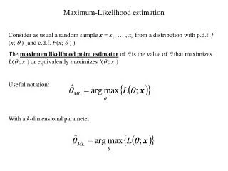
1. Maximum Likelihood Estimation of Mixture Densities for Binned and Truncated Multivariate Data Igor V. Cadez, Padhraic Smyth, Geoff J. Mclachlan, Christine and E. McLaren, Machine Learning 2001 (to appear) O, Jangmin 2001/06/01

2. Introduction (1) • Fitting mixture models to binned and truncated data by ML via EM. • Binning • measurement with finite resolution • quantifying real-valued variables • Truncation • Motivation • diagnostic evaluation of anemia • volume of RBC, amount of hemoglobin : measured by cytometric blood cell counter (Bayer Corp.)

3. Figure 1

4. Introduction (2) • Data in the form of histogram • Computer Vision, Massive data sets, … • Binning • Measurement Precision • Truncation • Limitation of the range of measurement, intentionally, … • EM frame work • Missing data: original data points.

5. Binned and Truncated Data • Sample space • v mutually exclusive regions Hr (r=1,…,v) • Observation • Only the number of nr of the Yj that fall in Hr (r=1,…,v0) is recorded (v0 v). • Observed data vector : • a is multinomial distribution

6. Observed log likelihood

7. Application of EM Algorithm : Missing Data • Unobservable frequencies in the case of truncation. • nr unobservable individuals in the rth region Yr. • Complete Data vector

8. p(a;) is specified • p(u|a;) can be specified… (negative binomial ?) • p(y1+,…, yv+|u, a; ) is specified • Conditioning on u and a, yj+ is composed by independent nj sampling from the density

9. Application of EM Algorithm : Missing Data • Then, complete data log-likelihood

10. Application of EM Algorithm : Mixture Model • Extension to mixture model (g components) • Conditional probability that Yrs belongs to i-th component given yrs. • Final complete data log-likelihood Zero-one indicator variable

11. E-Step • Calculation of Q(; (k)) • expection over y1+,…,yv+ • expection over u . • Expectation of u given a …

12. M-Step • i(k+1) update •  = (1,…, g) : other parameters are adjusted to be…

13. M-Step for Normal Components • Parameter update equation • Practical implementation is more complex due to multinomial integrals.

14. Computational and Numerical Issues • Integration can’t be evaluated analytically. • m bins in univariate, O(md) in d-dimensional. • O(i) evaluation in univariate integration, O(id) in d-dimensional • Complex geometry. • For fixed sample size, more sparser multivariate histogram • Integrating methods • Numerical • Monte Carlo • Romberg : Idea – repeated 1-dimensional integration.

15. Handling Truncated Regions • A single bin • No extra integration is needed.

16. 3.3 The Complete EM Algorithm • Treat the histogram as a PDF and draw a small number of data points from it • Fit the mixture model using the standard EM algorithm (nonbinned , nontruncated) • Using the parameter estimates from above, refine the estimate with the full EM algorithm applied to the binned and truncated data

17. 4. Experimental Results with Simulated Data • 3 experiments • Generate data from a known PDF and then bin them (bivariate). • Number of bin per dimension: 5 ~ 100 (step 5) • 10 different samples for smoothing results. • Standard EM on unbinned samples v.s. full EM on binned samples • Estimation method: KL distance between true density v.s. 2 EMs

18. Experiment Setup • To test the quality of the solution for different numbers of data points from Figure 4. • Data points N : 100 ~ 1000 (step 10) • (20 bin, 100 data, 10 samples) • To test performance of the algorithm when the component densities are not so well separated. • 3 apart components • (20 bin, 20 separation, 10 samples) • To test the performance of the algorithm when significant truncation occurs • (20 bin, 100 positions, 10 samples)

21. 4.2 Estimation from Random Samples Generated from the Binned Data • Baseline approach • Estimate PDF from a random sample from the binned data • Uniform sampling estimation method • Figure 6 : comparison • Overestimates the variance • Variance inflation

22. Figure 6 : Estimated PDFs obtained from original data and PDFs fitted by binned and the uniform random-sample algorithm for (a) 5 bins per dimension and (b) 10 per dimension. 3-covariance ellipse

23. 4.3 Experiments with Different Sample Size • Figure 7 • As a function of number of bins and number of data points • Bin > 20, data > 500 : small KL distance • Figure 8 • As a function of number of bins • Bin (5 ~ 20): rapid decay, Bin > 20 : flat • Figure 9 • As a function of number of data • Exponential decay

24. Figure 7 : (a) average KL distance between the estimated density and the true density, (b) standard deviation of the KL distance from10 repeated samples.

27. 4.4 Experiments with Different Separations of Mixture Components • Figure 10 • As a function of number of bins and separation of mean • Insensitive to separation of components • Figure 11 • As a function of separation of mean • Ratio of KL distance of the standard and binned algorithm • Small number of bin : standard EM is better. • Small separation : binned EM is better • Figure 12

31. 4.5 Experiments with Truncation • Figure 13 • Function of ratio of truncated points • Standard EM ignores the information of truncation • Relatively insensitive to truncation, in binned EM • Figure 14

34. Real Example : Red Blood Cell Data • Medical diagnosis • based on two-dimensional histograms characterizing RBC and hemoglobin measurements • Mixture densities were fitted to histograms from 90 control subject and 82 subjects with iron deficient anemia • B=1002, N=40,000 • Using for discriminant rule • Baseline features: 4-dim feature vector (mean, variance along RBC and hemoglobin) • 11-dim features: two-component lognormal mixture models (mean, cov, mixing weight) • 9-dim features: (mean, log-odds of eigenvalues of cov, mixing weight)

35. Figure 15. Contour plots from estimated density estimates for three control patients and three iron deficient anemia patients.

37. Conclusion • Fitting mixture densities to multivariate binned and truncated data • Computational and numerical implementation issues • In 2-dim simulation, If number of bins exceeds 10 the loss of information from quantization is minimal.