Mobile Radio Propagation
Mobile Radio Propagation. Mobile radio channel is an important factor in wireless systems. Wired channels are stationary and predictable, while radio channels are random and have complex models . Modeling of radio channels is done in statistical fashion based on receiver measurements.

Mobile Radio Propagation
E N D
Presentation Transcript
Mobile Radio Propagation • Mobile radio channel is an important factor in wireless systems. • Wired channels are stationary and predictable, while radio channels are random and have complex models. • Modeling of radio channels is done in statistical fashion based on receiver measurements.
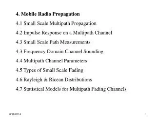
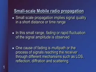
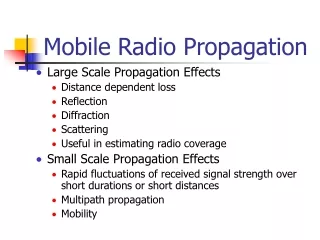
Types of propagation models • Large scale propagation models • To predict the averagesignal strength at a given distance from the transmitter • Controlled by signal decay with distance • Small scale or fading models. • To predict the signal strength at close distance to a particular location • Controlled by multipath and Doppler effects.
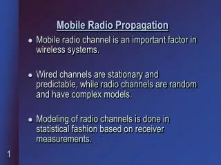
-30 -40 Received Power (dBm) -50 -60 -70 14 16 18 20 22 24 26 28 T-R Separation (meters) Radio signal pattern
Measured signal parameters • Electrical Field (Volts/m) Magnitude E = IEI Vector Direction E = xEx + yEy + zEz • Power (Watts or dBm) Power is scalar quantity and easier to measure.
Relation between Watts and dBm • P (dBm) = 10 log10 [P(mW)]
Physical propagation models • Free Space Propagation • Transmitter/receiver have clear LOS path • Reflection • Wave reaches receiver after reflection off surfaces larger than wavelength • Diffraction • Wave reaches receiver by bending at sharp edges (peaks) or curved surfaces (earth). • Scattering • Wave reaches receiver after bouncing off objects smaller than wavelength (snow, rain).
Free Space Propagation • Transmitter and receiver have clear, unobstructed LOS path between them. (Courtesy: webbroadband.blogspot.com)
Friistransmission equation Pr = PtGt Gr2 (4)2 d2 L Pt= Transmitted Power (W) Pr = Received Power (W) Gt= Transmitter antenna gain Gr = Receiver antenna gain L = System loss factor • Due to line losses, but not due to propagation • L 1
Antenna Gain • Power Gain of antenna G = 4Ae / 2, • Ae is effective aperture area of antenna • Wavelength = c / f (Hz) = 3 • 108 / f , meters
Relation between Electric field and Power • Received power Pr= IErI2 2 Gr 4 • Impedance of medium: = / • For air or vacuum: = (4 • 10-7) /(8.85 • 10-12 ) = 377
Example If the received power is Pr = 7 • 10-10 W, antenna gain Gr = 2 and transmitting frequency is 900 MHz, determine the electric field strength at the receiver.
Solution f = 900 MHz => = (3 • 108) / (900 • 106) = 0.33 m From field-power equation: IErI = [(Pr • • 4) / ( 2 • Gr)]1/2 = [(7 • 10-10• 377 • 4) / (0.332 • 2)]1/2 = 0.0039 V/m
Example A transmitter produces 50W of power. If this power is applied to a unity gain antenna with 900 MHz carrier frequency, find the received power at a LOS distance of 100 m from the antenna. What is the received power at 10 km? Assume unity gain for the receiver antenna.
Solution Pr = PtGt Gr2 (4)2 d2 L Pt = 50 W, Gt = 1, Gr = 1, L = 1, d = 100 m = (3 • 108) / (900 • 106) = 0.33 m Solving, Pr = 3.5 • 10-6 W Pr (10 km) = Pr (100 m) • (100/10000)2 = 3.5 • 10-6 • (1/100)2 = 3.5 • 10-10 W
Electric Properties of Material Bodies • Fundamental constants Permittivity = 0r , Farads/m Permeability = 0r ,Henries/m Conductivity ,Siemens/m • Types of materials • Dielectrics – allow EM waves to pass • Conductors – block EM waves • Metamaterials – bend EM waves
Reflection at dielectric boundaries Er = : Reflection coefficient Et = T = 1 + : Transmission coefficient Ei Ei Er Ei i r i= r Et
Vertical Polarization Ei Er Hi Hr 1, 1, 1 i r 2, 2, 2 t Et ||= 2sint - 1sini 2sint + 1sini
Horizontal Polarization Ei Er Hi Hr 1, 1, 1 i r 2, 2, 2 t Et T = 2sint - 1sini 2sint + 1sini
Reflection from Perfect Conductor (ET =0) Vert. polarizationHoriz. polarization i=ri=r Ei = ErEi = - Er Ei Er i r Et
Ground Reflection (2-Ray Model) T (transmitter) ETOT = ELOS +Eg ELOS Ei R (receiver) ht Er=Eg hr i 0 d
Field Equations d = several kms ht = 50-100m ETOT= ELOS + Eg ETOT(d) = For d > 20hthr / Received power Pr=
Example A mobile is located 5 km away from a base station, and uses a vertical /4 monopole antenna with a gain of 2.55dB to receive cellular radio signals. The electric field at 1 km from the transmitter is measured to be 10-3 V/m. The carrier frequency used is 900 MHz. (a) Find the length and gain of the receiving antenna.
Example A mobile is located 5 km away from a base station, and uses a vertical /4 monopole antenna with a gain of 2.55dB to receive cellular radio signals. The electric field at 1 km from the transmitter is measured to be 10-3 V/m. The carrier frequency used is 900 MHz. (b) Find the received power at the mobile using the 2-way ground model assuming the height of the transmitting antenna is 50 m and receiving antenna is 1.5 m above the ground.
Solution: d0 = 1 km E0 = 10-3 V/m ht = 50 m hr = 1.5 m d = 5 km
(a) f = 900 MHz = (3 • 108) / (900 • 106) = 0.33 m Length of receiving antenna, L = / 4 = 0.33/4 = 0.0833 m = 8.33 cm
(b) Gain of antenna = 2.55 dB = > 1.8 Er (d) = = 2 • 10-3 • 1 • 103 • 2 • 50 • 1.5 (5 • 103)2 • 0.333 = 113.1 • 10-6 V/m
Pr (d) = I Er I22 Gr 4 = (113.1 • 10-6) 2 • (0.333) 2 • 1.8 377 4 = 5.4 • 10-13 W = -92.68 dBm
Diffraction • Diffraction allows radio signals to propagate around the curved surface or propagate behind obstructions. • Based on Huygen’s principle of wave propagation.
R T h d2 d1 ht hr hobs Knife-edge Diffraction Geometry (a) T is transmitter and R is receiver, with an infinite knife-edge obstruction blocking the line-of-sight path.
T h h’ R d1 d2 ht hr Knife-edge Diffraction Geometry (b) T & R are not the same height...
T h h’ R d1 d2 ht hr Knife-edge Diffraction Geometry ...If and are small and h<<d1 and d2, then h & h’ are virtually identical and the geometry may be redrawn as in (c).
Knife-edge Diffraction Geometry (c) Equivalent where the smallest height (in this case hr ) is subtracted from all other heights. T ht-hr hobs-hr R d2 d1
Assumptions h << d1, d2 h >> Excess path length
...Assumptions h << d1, d2 h >> Phase difference = 2 / = 2 h2 (d1 + d2 ) 2 d1 d2
Diffraction Parameter v = =
Three Cases • Case I: h > 0 • Case II: h = 0 • Case III: h < 0
Case I: h > 0 and are positive since h is positive. h T R d1 d2
Case II: h = 0 and equal 0, since h equals 0. d1 d2 T R
Case III: h < 0 and are negative, since h is negative. d1 d2 T R h
The electric field strength of the diffracted wave is given by: Ed = F(v) • Eo where Eois the free space field strength in the absence of both ground and knife edge.
Approximate Value of Fresnel Integral F(v): Gd(dB) = 20log IF(v)I
v Range Gd (dB) v -1 0 -1v 0 20 log (0.5 – 0.62 v) 0v1 20 log (0.5 e-0.95v) 1v2.4 20 log (0.4 – v2.4 20 log (0.225 /v)
Example Compute the diffraction loss between the transmitter and receiver assuming: = 1/3m d1 = 1km d2 = 1km h = 25m
Solution: Given = 1/3 m d1 = 1km d2 = 1km h = 25m V = = = 2.74
Using the table, Gd (dB) = 20 log (0.225/2.74) = -22 dB Loss = 22 dB
Scattering • When a radio wave impinges on a rough surface, the reflected energy is spread out or diffused in all directions. Ex., lampposts and foliage. • The scattered field increases the strength of the signal at the receiver.
Radar Cross Section (RCS) Model RCS (Radar Cross Section) = Power density of scattered wave in direction of receiver Power density of radio wave incident on the scattering object
Radar Cross Section (RCS) Model PR = PT • GT • 2 • RCS (4)3 • dT 2 • dR 2 Where, PT = Transmitted Power GT = Gain of Transmitting antenna dT = Distance of scattering object from Transmitter dR = Distance of scattering object from Receiver
Practical Link Budget • Most radio propagation models are derived using a combination of analytical and empirical models. • Empirical approach is based on fitting curves or analytical expressions that recreate a set of measured data.
...Practical Link Budget • Advantages of empirical models; Takes into account all propagation factors, both known and unknown. • Disadvantages:New models need to be measured for different environment or frequency.