Space Weather Prediction: Challenges in Computational Magnetohydrodynamics
400 likes | 633 Vues
Space Weather Prediction: Challenges in Computational Magnetohydrodynamics. Gábor Tóth Center for Space Environment Modeling University of Michigan. Collaborators. Tamas Gombosi, Kenneth Powell Ward Manchester, Ilia Roussev Darren De Zeeuw , Igor Sokolov Aaron Ridley, Kenneth Hansen

Space Weather Prediction: Challenges in Computational Magnetohydrodynamics
E N D
Presentation Transcript
Space Weather Prediction: Challenges in Computational Magnetohydrodynamics • Gábor Tóth • Center for Space Environment Modeling • University of Michigan
Collaborators • Tamas Gombosi, Kenneth Powell • Ward Manchester, Ilia Roussev • Darren De Zeeuw, Igor Sokolov • Aaron Ridley, Kenneth Hansen • Richard Wolf, Stanislav Sazykin (Rice University) • József Kóta (Univ. of Arizona) Grants DoD MURI and NASA CT Projects
Outline of Talk • What is Space Weather and Why to Predict It? • Parallel MHD Code: BATSRUS • Space Weather Modeling Framework (SWMF) • Some Results • Concluding Remarks
What Space Weather Means Conditions on the Sun and in the solar wind, magnetosphere, ionosphere, and thermosphere that can influence the performance and reliability of space-born and ground-based technological systems and can endanger human life or health. Space physics that affects us.
MHD Code: BATSRUS • Block Adaptive Tree Solar-wind Roe Upwind Scheme • Conservative finite-volume discretization • Shock-capturing Total Variation Diminishing schemes • Parallel block-adaptive grid (Cartesian and generalized) • Explicit and implicit time stepping • Classical and semi-relativistic MHD equations • Multi-species chemistry • Splitting the magnetic field into B0 + B1 • Various methods to control the divergence of B
Conservative form is required for correct jump conditions across shock waves. Energy conservation provides proper amount of Joule heating for reconnection even in ideal MHD. Non-conservative pressure equation is preferred for maintaining positivity. Hybrid scheme: use pressure equation where possible. MHD Equations in Conservative vs. Non-Conservative Form
The magnetic field has huge gradients near the Sun and Earth: Large truncation errors. Pressure calculated from total energy can become negative. Difficult to maintain boundary conditions. Solution: split the magnetic field as B = B0 + B1 where B0 is a divergence and curl free analytic function. Gradients in B1 are small. Total energy containsB1 only. Boundary condition for B1 is simple. Splitting the Magnetic Field
Vastly Disparate Scales • Spatial: • Resolution needed at Earth:1/4 RE • Resolution needed at Sun:1/32 RS • Sun-Earth distance:1AU • 1 AU = 215 RS = 23,456 RE • Temporal: • CME needs 3 days to arrive at Earth. • Time step is limited to a fraction of a second in some regions.
Adaptive Block Structure Blocks communicate with neighbors through “ghost” cells Each block is NxNxN
Why Explicit Time-Stepping May Not Be Good Enough • Explicit schemes have time steplimited by CFL condition: Δt < Δx/fastest wave speed. • High Alfvén speeds and/or small cells may lead to smaller time steps than required for accuracy. • The problem is particularly acute near planets with strong magnetic fields. • Implicit schemes do not have Δt limited by CFL.
Building a Parallel Implicit Solver • BDF2 second-order implicit time-stepping scheme requires solution of a large nonlinear system of equations at each time step. • Newton linearization allows the nonlinear system to be solved by an iterative process in which large linear systems are solved. • Krylov solvers (GMRES, BiCGSTAB) with preconditioning are robust and efficient for solving large linear systems. • Schwarz preconditioning allows the process to be done in parallel: • Each adaptive block preconditions with based on local data • MBILU preconditioner
Getting the Best of Both Worlds - Partial Implicit • Fully implicit scheme has no CFL limit, but each iteration is expensive (memory and CPU) • Fully explicit is inexpensive for one iteration, but CFL limit may mean a very small Δt • Set optimal Δt limited by accuracy requirement: • Solve blocks with unrestrictive CFL explicitly • Solve blocks with restrictive CFL implicitly • Load balance explicit and implicit blocks separately
The Sun-Earth system consists of many different interconnecting domains that are independently modeled. Each physics domain model is a separate application, which has its own optimal mathematical and numerical representation. Our goal is to integrate models into a flexible software framework. The framework incorporates physics models with minimal changes. The framework can be extended with new components. The performance of a well designed framework can supercede monolithic codes or ad hoc couplings of models. From Codes To Framework
Solar CoronaSCBATSRUS Eruptive Event GeneratorEEBATSRUS Inner HeliosphereIH BATSRUS Solar Energetic ParticlesSPKóta’s SEP model Global Magnetosphere GM BATSRUS Inner MagnetosphereIM Rice Convection Model Ionosphere ElectrodynamicsIERidley’s potential solver Upper AtmosphereUA General Ionosphere Thermosphere Model (GITM) Physics DomainsID Models
Parallel Layout and Execution LAYOUT.in for 20 PE-s SC/IHGMIM/IE ID ROOT LAST STRIDE #COMPONENTMAP SC 0 9 1 IH 0 9 1 GM 10 17 1 IE 18 19 1 IM 19 19 1 #END
Stream line and field line tracing is a common problem in space physics. Two examples: Coupling inner and global magnetosphere models Coupling solar energetic particle model with MHD Tracing a line is an inherently serial procedure Tracing many lines can be parallelized,but Vector field may be distributed over many PE-s Collecting the vector field onto one PE may be too slow and it requires a lot of memory Parallel Field Line Tracing
Coupling Inner and Global Magnetosphere Models Pressure Inner magnetospheremodel: needs the field line volumes, average pressure and density along field lines connected to the 2D grid on the ionosphere. Global magnetosphere model: needs the pressure correction along the closed field lines:
Interpolated Tracing Algorithm 1. Trace lines inside blocks starting from faces. 2. Interpolate and communicate mapping. 3. Repeat 2. until the mapping is obtained for all faces. 4. Trace lines inside blocks starting from cell centers. 5. Interpolate mapping to cell centers.
4. Receive lines from other PE-s. 5. If received line go to 2a. Parallel Algorithm without Interpolation PE 1 PE 2 1.Find next local field line. 2. If there is a local field line then 2a. Integrate in local domain. 2b. If not done send to other PE. PE 3 PE 4 3. Go to 1. unless time to receive. 6. Go to 1. unless all finished.
Modeling a Coronal Mass Ejection • Set B0 to a magnetogram based potential field. • Obtain MHD steady state solution. • Use source terms to model solar wind acceleration and heating so that steady solution matches observed solar wind parameters. • Perturb this initial state with a “flux rope”. • Follow CME propagation. • Let CME hit the Magnetosphere of the Earth.
More Detail at Earth Pressure and magnetic field Before shock After shock Density and magnetic field at shock arrival time South Turning BZ North Turning BZ
Before shock hits. After shock: currents and the resulting electric potential increase. Region-2 currents develop. Although region-1 currents are strong, the potential decreases due to the shielding effect. Current Potential Ionosphere Electrodynamics
The Hall conductance is calculated by the Upper Atmosphere component and it is used by the Ionosphere Electrodynamics. After the shock hits the conductance increases in the polar regions due to the electron precipitation. Note that the conductance caused by solar illumination at low latitudes does not change significantly. Before shock arrival Upper Atmosphere After shock arrival
2003 Halloween Storm Simulation with GM, IM and IE Components • The magnetosphere during the solar storm associated with an X17 solar eruption. • Using satellite data for solar wind parameters • Solar wind speed: 1800 km/s. • Time: October 29, 0730UT • Shown are the last closed field lines shaded with the thermal pressure. • The cut planes are shaded with the values of the electric current density.
Concluding Remarks • The Space Weather Modeling Framework (SWMF) uses sate-of-the-art methods to achieve flexible and efficient coupling and execution of the physics models. • Missing pieces for space weather prediction: • Better models for solar wind heating and acceleration; • Better understanding of CME initiation; • More observational data to constrain the model; • Even faster computers and improved algorithms.