Download
1 / 19
190 likes | 222 Vues
This paper presents an adaptive FIR neural model for centroid learning in Self-Organizing Maps, optimizing filter parameters to minimize a cost function, improving convergence properties, and using a simplified neighborhood function. The Σ-matrix visualization tool is introduced for data visualization.

E N D
Adaptive FIR Neural Model for Centroid Learning in Self-Organizing Maps Mauro Tucci and Marco Raugi TNN, 2010 Presented by Wen-Chung Liao 2010/07/28
Outlines • Motivation • Objectives • Methodology • Model Analysis • The Σ-matrix Visualization Tool • Conclusions • Comments
Motivation • There are two different SOM algorithms: the sequential algorithm, and the batch algorithm. • The batch algorithm performs one order of magnitude faster • however it is not well suited to variants and generalizations as the sequential one
Objectives • A model of the SOM processing unit for the learning of static distributions is presented. • each neuron • a general filter model • a finite impulse response (FIR) system • optimize the parameters of the filter in order to minimize a cost function during the training. trace matrix FIR coefficients model vector
Objectives • The FIR process of each neuron tends to become a moving average filter. • gives an insight of the update rule of the classic SOM algorithm. • improves the convergence properties with respect to the classic SOM. • uses a neighborhood function with a simplified design, where the annealing scheme for the learning rate is not needed. • used to visualize a set of properties of the input data set
Methodology N: the order of the FIR filters
Methodology LMS algorithm LME algorithm Dm: a distortion measure of the SOM Step size: α
FIR-SOMComplete Learning Algorithm 1) Given the vector input data set to analyze Δ Rn, create the output grid array of a finite number of cells i=1,…, D. 2) Design a decreasing function for the neighborhood width σ(t), and choose the step size α, of the filter estimator.
FIR-SOMComplete Learning Algorithm 3) For each cell, initialize the trace matrix by using random or linear initialization. 4) Choose the order of the FIR filters and initialize the coefficients to zero 5) At each time step t=0, 1, 2,…, compute the model vector of each cell i=1,…, D as
FIR-SOMComplete Learning Algorithm 6) Pick at random one sample from the input data set Δ and find the BMU as where 7) Compute the filter coefficients, for i=1,…, D, with 8) Update the trace matrix for each cell i=1,…, D, with where 9) Increase the time step and return to 5), or stop if the maximum number of iterations has been reached. (LMS algorithm)
Model Analysis • FIR Coefficients Initialized by Zero Converge to 1/N • Δ1: distributed in gray square • 2-D 30x30 map • N=10 • T=40000
B. The Moving Average SOM • MA-SOM D. Convergence Properties of the MA-SOM C. Quality Indexes The topographic error TE(Δ)
MA-SOM shows better quantization errors of the basic SOM for the same training duration • Δ2: a Gaussian distribution • N=10 • the centroid neural network(CNN) • A practical algorithm for the computation of an optimal set of unordered centroids in multivariate data. • provides a guarantee of convergence to a local minimum of the quantization error. • CNN required higher computational times than MA-SOM
THE Σ-MATRIX VISUALIZATION TOOL LME algorithm • Σ-matrix • εi assumes higher values in correspondence of high-density zones • U-matrix • visualizing in each cell the mean of the distances between the model vector of the cell and those of the adjacent units, • P-matrix • based on Pareto density estimation (PDE) method • RD-matrix
RD-matrix U-matrix • Δ3 R6 • Two clusters, Gaussian distributions • 2-D 30x30 map • N=10 • LME algorithm with the FIR coefficients initialized to 1/N • T=40000 P-matrix Σ-matrix
Σ-matrix P-matrix • Δ4 R30 • Two clusters, one Gaussian distribution, one uniform distribution • 2-D 30x30 map • LME algorithm • N=10
Σ-matrix P-matrix • WINE • 178 labeled instances • 13 attributes • 3 types of wines • 2-D 30x30 map • N=10 • LME algorithm MA-SOM,Σ-matrix U-matrix
Conclusions • a good alternative to the classic SOM algorithm. • a reduced number of input presentations to reach a final state with improved map quality measures with respect to the classic SOM. • requires an added amount of basic operations and memory, but a shorter time duration of the training with respect to the classic SOM • the proposed neuron model is based onan adaptive structure, while in the classic SOM and other SOM variants, the neuron model is defined a priori. • the optimal FIR filters are moving average filters. • a proposed visualization technique, called Σ-matrix, which is based on the optimized FIR parameters.
Comments • Advantage • Good mapping quality • Good visualization tool • Shortage • The definition of model vector’s adaptation is a little ambiguous. • Applications • Clustering • Classification