Download

1 / 81
810 likes | 937 Vues
This research investigates the intricate relationship between X-ray emissions in massive stars and their magnetic fields. By understanding the physics behind magnetic fields in massive stars, we aim to leverage X-ray observations to identify and classify these stars, particularly those in the Orion Nebula Cluster. While diverse X-ray behaviors have been observed, our understanding of the mechanisms driving these X-ray emissions remains limited. Through detailed analysis of Chandra and XMM-Newton data, we explore current models and seek to uncover the underlying processes at play in massive stellar environments.

E N D
X-ray Diagnostics and Their Relationship to Magnetic Fields David CohenSwarthmore College
If we understand the physical connection between magnetic fields in massive stars and X-rays, we could use X-ray observations to identify magnetic massive stars. e.g. Which of the stars in this Chandra X-ray image of the Orion Nebula Cluster are massive magnetic stars?
But we’re not there yet… X-ray behavior of known magnetic massive stars is diverse. We don’t understand enough about the physical mechanisms of X-ray production in them.
Stellar rotation vs. X-ray luminosity low-mass stars high-mass stars No trend
X-rays in massive stars are associated with their radiation-driven winds
erg s-1 Power in these winds: while the x-ray luminosity To account for the x-rays, only one part in 10-4of the wind’s mechanical power is needed to heat the wind
Three models for massive star x-ray emission 1. Instability driven shocks 2. Magnetically channeled wind shocks 3. Wind-wind interaction in close binaries
Three models for massive star x-ray emission 1. Instability driven shocks 2. Magnetically channeled wind shocks 3. Wind-wind interaction in close binaries
What are these “X-rays” anyway? …and what’s the available data like?
Launched 2000: superior sensitivity, spatial resolution, and spectral resolution Chandra XMM-Newton sub-arcsecond resolution
Both have CCD detectors for imaging spectroscopy: low spectral resolution: R ~ 20 to 50 Chandra XMM-Newton And both have grating spectrometers: R ~ few 100 to 1000 300 km/s
The gratings have poor sensitivity… We’ll never get spectra for more than two dozen hot stars Chandra XMM-Newton
The Future: Chandra XMM-Newton Astro-H (Japan) – high spectral resolution at high photon energies …few years from now International X-ray Observatory (IXO)… 2020+
ChandraACISOrion Nebula Cluster (COUP) q1Ori C Color coded according to photon energy (red: <1keV;green 1 to 2 keV; blue > 2 keV)
q1Ori C: X-ray lightcurve Stelzer et al. 2005 not zero
sOri E: XMM light curve Sanz-Forcada et al. 2004
XMM EPIC spectrum of sOri E Sanz-Forcada et al. 2004
Chandra grating spectra: 1 Ori C and a non-magnetic O star 1 Ori C z Pup
thermal emission “coronal approximation” valid: electrons in ground state, collisions up, spontaneous emission down optically thin lines from highly stripped metals, weak bremsstrahlung continuum (continuum stronger for higher temperatures)
thermal emission “coronal approximation” valid: electrons in ground state, collisions up, spontaneous emission down optically thin lines from highly stripped metals, weak bremsstrahlung continuum (continuum stronger for higher temperatures)
thermal emission “coronal approximation” valid: electrons in ground state, collisions up, spontaneous emission down optically thin lines from highly stripped metals, weak bremsstrahlung continuum (continuum stronger for higher temperatures)
thermal emission “coronal approximation” valid: electrons in ground state, collisions up, spontaneous emission down optically thin lines from highly stripped metals,weak bremsstrahlung continuum (continuum stronger for higher temperatures)
Chandra grating spectra: 1 Ori C and a non-magnetic O star 1 Ori C z Pup
Energy Considerations and Scalings 1 keV ~ 12 × 106 K ~ 12 Å Shock heating: Dv = 300 km/sgives T ~ 106 K (and T ~ v2) ROSAT 150 eV to 2 keV Chandra, XMM 350 eV to 10 keV
Energy Considerations and Scalings 1 keV ~ 12 × 106 K ~ 12 Å Shock heating: Dv = 1000 km/sgives T ~ 107 K (and T ~ v2) ROSAT 150 eV to 2 keV Chandra, XMM 350 eV to 10 keV
1 Ori C z Pup H-like/He-like ratio is temperature sensitive Mg XII Mg XI Si XIV Si XIII
1 Ori C z Pup 1Ori C – is hotter Mg XII Mg XI Si XIV Si XIII H/He > 1 in 1Ori C
Differential Emission Measure (temperature distribution) q1Ori C is much hotter Wojdowski & Schulz (2005)
q1 Ori C(O7 V) z Pup(O4 If) Emission lines are significantly narrower, too 1000 km s-1
Ne X Ly-a in q1Ori C : cooler plasma, broader – some contribution from “standard” instability wind shocks
Dipole magnetic field Wade et al. 2008
What about confinement? Recall: q1Ori C: h* ~ 20 : decent confinement
What about confinement? Recall: zOri: h* ~ 0.1 : poor confinement q1Ori C: h* ~ 20 : decent confinement sOri E: h* ~ 107 : excellent confinement
Simulation/visualization courtesy A. ud-DoulaMovie available at astro.swarthmore.edu/~cohen/presentations/apip09/t1oc-lowvinf-logd.avi
Simulation/visualization courtesy A. ud-DoulaMovie available at astro.swarthmore.edu/~cohen/presentations/apip09/t1oc-lowvinf-logT.avi
Simulation/visualization courtesy A. ud-DoulaMovie available at astro.swarthmore.edu/~cohen/presentations/apip09/t1oc-lowvinf-speed.avi
MHD simulations of magnetically channeled wind temperature emission measure simulations by A. ud-Doula; Gagné et al. (2005) Channeled collision is close to head-on:Dv > 1000 km s-1 : T > 107 K
Differential emission measure (temperature distribution) MHD simulation of 1Ori C reproduces the observed differential emission measure Wojdowski & Schulz (2005)
0.4 1.5 0.3 1.0 Simulation EM (1056 cm-3) 0.2 θ1 Ori C ACIS-I count rate (s-1) 0.5 0.1 0.0 0.0 0.0 0.2 0.4 0.6 0.8 1.0 Rotational phase (P=15.422 days) Chandra broadband count rate vs. rotational phase Model from MHD simulation