Association Mapping
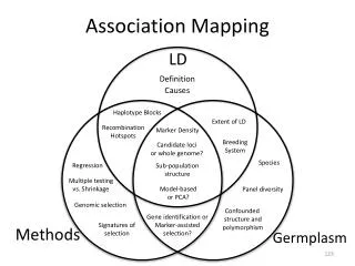
Association Mapping. LD. Definition. Causes. Haplotype Blocks. Extent of LD. Recombination Hotspots. Marker Density. Breeding System. Candidate loci or whole genome?. Species. Regression. Sub-population structure. Multiple testing vs. Shrinkage. Model-based or PCA?.

Association Mapping
E N D
Presentation Transcript
Association Mapping LD Definition Causes Haplotype Blocks Extent of LD Recombination Hotspots Marker Density Breeding System Candidate loci or whole genome? Species Regression Sub-population structure Multiple testing vs. Shrinkage Model-based or PCA? Panel diversity Genomic selection Confounded structure and polymorphism Gene identification or Marker-assisted selection? Signatures of selection Methods Germplasm
Outline • Association mapping is regression • Accounting for structure • Estimating structure using markers • Truly multi-factorial models • Miscelaneous topics: • Genomic control; TDT; Confounding with structure; Haplotype predictors; Genetic heterogeneity; Missing heritability; NAM; Validation
Association Mapping • It’s the same thing as linkage mapping in a bi-parental population but in a population that has not been carefully designed and generated experimentally • Because the experiment has not been designed, it is messy. Statistical methods are needed to deal with the mess
Regression • xiis the allelic state at a marker • Consider the total genotypic effect of I • qi is the allelic state at a QTL with which the marker is (hopefully) in LD • Now estimate β
Estimate of Beta Part having to do with LD Multi-factorialtrait / structure
When is cov(x, g) non-zero? • Differences in allele frequencies at the marker between subpopulations AND difference in phenotypic mean between subpopulations • The difference in mean can be due to a single or many loci • Difference in the frequency of alleles between families AND difference in family phenotypic means within a (sub)population
Structure possibilities Population structure Familial relatedness Yu, J., Pressoir, G., et al. 2006. Nat Genet 38:203-208
Controlling for structure • Basic quantitative genetics: • Two individuals who share many alleles should resemble each other phenotypically • Use markers to figure out how many alleles individuals share and then use that to adjust statistically for their phenotypic resemblance
Controlling for structure • The “mixed model” Yu, J., Pressoir, G., et al. 2006. Nat Genet 38:203-208
Controlling for structure • Structure => large differences in allele frequencies across many markers Potential Phenotypic Gradient First PCA axis Regression coefficients of the phenotype on the PCA values
Use of PCA • Results are not sensitive to the number of PCA, provided you have enough • Price, A.L. et al. 2006. Principal components analysis corrects for stratification in genome-wide association studies. Nat Genet 38:904-909 • The number of significant PC can be determined • Patterson, N. et al. 2006. Population Structure and Eigenanalysis. PLoS Genetics 2:e190 • Use a “Screeplot”
Historical footnote • PCA achieves what the Pritchard program Structure does • PCA is faster and more robust Pritchard, J.K. et al. 2000. Genetics 155:945-959 Price A.L. et al. 2006. Nat Genet 38:904-909. Patterson N. et al. 2006. PLoS Genetics 2:e190
Kinship • We are all a little bit related: • Two unrelated people: go back 1 generation, all four parents must be different people. • Go back 2 generations, all eight grand-parents must be different people. • Go back 30 generations, all 2.1 billion ancestors would need to be different people: Impossible!
Identity by Descent • Two alleles that are copies (through reproduction) of the same ancestral allele Coefficient of Coancestry • Choose a locus • Pick an allele from Ed and one from Peter • Probability that the alleles are IBD = Ed and Peter’s Coefficient of Coancestry, θEP
Coef. of Coancestry –> A matrix • A is the additive relationship or kinship matrix Winter Six-Row “Bison” Two-Row
A constrains u • Two individuals who share many alleles should resemble each other phenotypically • u is the polygenic effect • Its covariance matrix is Var(u) = Aσ2u • If aij has a high value, the ui and uj should have similar values (they have high covariance) • A constrains the values that are possible for u
A matrix from the pedigree • The cells in the A matrix are aij = 2θij, the additive relationship coefficients between i in the row and j in the column • Coefficient of coancestryθij: the prob that a random alleles from i and j are IBD • Calculate from the pedigree by recursion:
A matrix from marker data , the homozygosities over all markers and alleles
With inbreeding, parental contributions NOT 50:50 / Maize intermated population Drift during intermating and inbreeding Markers can give more accurate θ than pedigree
Mixed Model Example • Five individuals, a, b, c, d, and e. • a and b in subpop 1; c, d, and e in subpop2. • a, b, c, and d unrelated; e is offspring of c and d. • a and d carry the 0; b, c, and e carry the 1 allele y = μ + Xβ + Qv
Mixed Model Example • Five individuals, a, b, c, d, and e. • a and b in subpop 1; c, d, and e in subpop2. • a, b, c, and d unrelated; e is offspring of c and d. • a and d carry the 0; b, c, and e carry the 1 allele y = μ + Xβ + Qv
Mixed Model Example • Five individuals, a, b, c, d, and e. • a and b in subpop 1; c, d, and e in subpop2. • a, b, c, and d unrelated; e is offspring of c and d. • a and d carry the 0; b, c, and e carry the 1 allele + Qv + Zu + e y = μ + Xβ
Mixed Model Example • Five individuals, a, b, c, d, and e. • a and b in subpop 1; c, d, and e in subpop2. • a, b, c, and d unrelated; e is offspring of c and d. • a and d carry the 0; b, c, and e carry the 1 allele Zu A = var(u) = σ2u
Mixed Model Example • There is a polygenic effect ufor each individual => overdetermined model? • NO: u is a random effect, constrained by Aσ2u
Mixed Model Example + Qv y = μ + Xβ + Zu + e –1 = ✕
Flowering time (High population structure) Ear height (Moderate population structure) Ear diameter (Low population structure) 0.5 0.5 0.5 a. b. c. 0.4 Simple Simple 0.4 Q 0.4 Q K GC Q Q + K 0.3 0.3 0.3 Q + K Simple Cumulative P K K 0.2 0.2 0.2 Q + K GC 0.1 0.1 0.1 GC 0 0 0 0 0.1 0.2 0.3 0.4 0.5 0 0.1 0.2 0.3 0.4 0.5 0 0.1 0.2 0.3 0.4 0.5 Observed P Observed P Observed P Simple Q K Q + K GC Control false positives from structure A straight diagonal line indicates an appropriate control of false positives. Q + K model has best Type I error control, most important when trait is related to population structure (e.g., flowering time).
Flowering time (High population structure) Ear height (Moderate population structure) Ear diameter (Low population structure) 1 1 1 d. e. f. K Q Q + K Q + K 0.8 0.8 0.8 Q + K K Q Q Simple Simple 0.6 0.6 0.6 Adjusted average power K Simple GC GC 0.4 0.4 0.4 Simple GC Q K 0.2 0.2 0.2 Q + K GC 0 0 0 0 0.2 0.4 0.6 0.8 1 0 0.2 0.4 0.6 0.8 1 0 0.2 0.4 0.6 0.8 1 (0) (0.8) (3.3) (7.1) (11.9) (17.4) (0) (0.8) (3.3) (7.1) (11.9) (17.4) (0) (0.8) (3.3) (7.1) (11.9) (17.4) Genetic effect Genetic effect Genetic effect (Phenotypic variation explained in %) (Phenotypic variation explained in %) (Phenotypic variation explained in %) Statistical power Q + K model had highest power to detect SNPs with true effects.
Controlling for Structure Original P Matrix K Matrix
Take homes on diversity • At equal population size • A less diverse population can increase power because relative to the extent of LD, the average marker distance is lower • Given that you are testing fewer markers, the multiple testing problem is reduced • Avoid as much as possible reducing population size for the sake of obtaining a more homogeneous population
Guidelines • More lines and more markers are better • For a diverse population, 800+ lines • For a narrower population, 300+ (?) • FDR is a reasonable method of determining significance, but probably conservative
Q constant K estimated • Q estimated with all markers, K estimated with varying fraction of markers available Flowering time Ear height Ear diameter d e f Variance ratio SSR SNP Marker number Marker number Marker number
Q estimated K constant • Q estimated with varying fraction of markers available, K estimated with all markers Flowering time Ear height Ear diameter d e f Variance ratio SSR SNP Marker number Marker number Marker number
History / future of controlling for structure Part having to do with LD Multi-factorialtrait / structure
Single locus: model mis-specification • “the problem is better thought of as model mis-specification: when we carry out GWA analysis using a single SNP at a time, we are in effect modeling a multifactorial trait as if it were due to a single locus” • Atwell S. et al. 2010. Nature 465:627-631
History: Candidate locus studies • AM started out with candidate locus studies where the effects of few loci could be fitted • The biotechnology was not there to type more than a few loci • The genetic background needed to be accounted for somehow (see above) • In any event, the computational power was not there to fit all 106 loci simultaneously
Future: GWAS fitting all loci • These methods could displace mixed models accounting for structure Logsdon B. et al. 2010.BMC Bioinformatics 11:58.
Sundry topics • Other methods to control structure • QTL confounded with structure • Single markers or haplotypes? • Genetic heterogeneity • Missing heritability • Linkage disequilibrium / Linkage analysis • Validation
Genomic Control • Calculate bias in distribution of test statistic using “neutral” loci, then account for bias • Devlin, B. and Roeder, K. 1999. Genomic Control for Association Studies. Biometrics 55:997-1004. • Works best for candidate genes: test loci can be distinguished from neutral control loci. Works less well for whole genome scans • Marchini, J. et al. 2004. Nat. Genet. 36:512-517 • Devlin, B. et al. 2004. Nat. Genet. 36:1129-1131. • Marchini, J. et al. 2004. Nat. Genet. 36:1131-1131
Transmission Disequilibrium Test • Experimental rather than statistical control of effects of structure • Originally conceived for dichotomous (e.g., disease / no disease) traits • Affected offspring and both parents, of which one must be heterozygous • Test whether the a putative causal allele is transmitted more often that 50% of the time • Spielman, R.S. et al. 1993. Am. J. Hum. Genet. 52:506-516
TDT • Extensions for quantitative traits • Allison, D.B. 1997. Am. J. Hum. Genet. 60:676-690 • Extensions for larger-than-trio pedigrees • Monks, S.A., and N.L. Kaplan. 2000. Am J Hum Genet 66:576-92 • Using for populations under artificial selection • Bink, M.C.A.M. et al. 2000. Genetical Res. 75:115-121
QTL confounded with structure • Particularly important for QTL affecting adaptation, e.g., flowering time Camus-Kulandaivelu, L. et al. 2006. Genetics 172:2449–2463
Also in rice… Ghd7-0aNon-functional Given geographic distribution and role in adaptation, selection using this locus will have marginal utility Ghd7-2Weak allele Ghd7-0Deleted Ghd7-1, Ghd7-3Functional Xue, W. et al. 2008. Nat Genet 40:761-767
Confounded QTL with structure • Association analysis will have difficulty identifying such QTL: the QTL needs to be polymorphic within subpopulations • Traditional linkage studies of crosses between members of different subpopulations should be very effective in this case • e.g., Xue, W. et al. 2008. Nat Genet 40:761-767 • Multi-factorial methods will have difficulty identifying loci under strong structure
Dwarf8: Confounded with structure • Thornsberry, J.M. et al. 2001. Nat. Genet. 28:286-289 • First structured association test applied to plants Camus-Kulandaivelu, L. et al. 2006. Genetics 172:2449–2463
Single markers or haplotypes? • The jury is still out • Infinite ways to simulate and analyze • Ne, QTL MAF, QTL effect, quantitative vs. binary, age of mutation • Ex. 1: Dramatically more power for haplotypesvs single markers • Durrant, C. et al. 2004. Am J Hum Genet 75:35-43
Single markers or haplotypes? • Ex. 2: Similar or lower power for haplotype method relative to single marker method • Zhao, H.H. et al. 2007. Genetics 175:1975-1986 • Process to sort out what method most appropriate for when still has to happen