Download
1 / 44
450 likes | 611 Vues
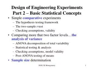
Design of Engineering Experiments Part 2 – Basic Statistical Concepts. Simple comparative experiments The hypothesis testing framework The two-sample t -test Checking assumptions, validity Comparing more that two factor levels… the analysis of variance

E N D
Design of Engineering ExperimentsPart 2 – Basic Statistical Concepts • Simple comparative experiments • The hypothesis testing framework • The two-sample t-test • Checking assumptions, validity • Comparing more that two factor levels…theanalysis of variance • ANOVA decomposition of total variability • Statistical testing & analysis • Checking assumptions, model validity • Post-ANOVA testing of means • Sample size determination DOX 5E Montgomery
Portland Cement Formulation (Table 2-1, pp. 22) DOX 5E Montgomery
Graphical View of the DataDot Diagram, Fig. 2-1, pp. 22 DOX 5E Montgomery
Box Plots, Fig. 2-3, pp. 24 DOX 5E Montgomery
The Hypothesis Testing Framework • Statistical hypothesis testing is a useful framework for many experimental situations • Origins of the methodology date from the early 1900s • We will use a procedure known as the two-sample t-test DOX 5E Montgomery
The Hypothesis Testing Framework • Sampling from a normal distribution • Statistical hypotheses: DOX 5E Montgomery
Estimation of Parameters DOX 5E Montgomery
Summary Statistics (pg. 35) Formulation 2 “Original recipe” Formulation 1 “New recipe” DOX 5E Montgomery
How the Two-Sample t-Test Works: DOX 5E Montgomery
How the Two-Sample t-Test Works: DOX 5E Montgomery
How the Two-Sample t-Test Works: • Values of t0 that are near zero are consistent with the null hypothesis • Values of t0 that are very different from zero are consistent with the alternative hypothesis • t0 is a “distance” measure-how far apart the averages are expressed in standard deviation units • Notice the interpretation of t0 as a signal-to-noiseratio DOX 5E Montgomery
The Two-Sample (Pooled) t-Test DOX 5E Montgomery
The Two-Sample (Pooled) t-Test • So far, we haven’t really done any “statistics” • We need an objective basis for deciding how large the test statistic t0 really is • In 1908, W. S. Gosset derived the referencedistribution for t0 … called the t distribution • Tables of the t distribution - text, page 640 DOX 5E Montgomery
The Two-Sample (Pooled) t-Test • A value of t0 between –2.101 and 2.101 is consistent with equality of means • It is possible for the means to be equal and t0 to exceed either 2.101 or –2.101, but it would be a “rareevent” … leads to the conclusion that the means are different • Could also use the P-value approach DOX 5E Montgomery
The Two-Sample (Pooled) t-Test • The P-value is the risk of wrongly rejecting the null hypothesis of equal means (it measures rareness of the event) • The P-value in our problem is P = 3.68E-8 DOX 5E Montgomery
Minitab Two-Sample t-Test Results Two-Sample T-Test and CI: Form 1, Form 2 Two-sample T for Form 1 vs Form 2 N Mean StDev SE Mean Form 1 10 16.764 0.316 0.10 Form 2 10 17.922 0.248 0.078 Difference = mu Form 1 - mu Form 2 Estimate for difference: -1.158 95% CI for difference: (-1.425, -0.891) T-Test of difference = 0 (vs not =): T-Value = -9.11 P-Value = 0.000 DF = 18 Both use Pooled StDev = 0.284 DOX 5E Montgomery
Checking Assumptions – The Normal Probability Plot DOX 5E Montgomery
Importance of the t-Test • Provides an objective framework for simple comparative experiments • Could be used to test all relevant hypotheses in a two-level factorial design, because all of these hypotheses involve the mean response at one “side” of the cube versus the mean response at the opposite “side” of the cube DOX 5E Montgomery
Confidence Intervals (See pg. 42) • Hypothesis testing gives an objective statement concerning the difference in means, but it doesn’t specify “how different” they are • Generalform of a confidence interval • The 100(1- )% confidenceinterval on the difference in two means: DOX 5E Montgomery
What If There Are More Than Two Factor Levels? • The t-test does not directly apply • There are lots of practical situations where there are either more than two levels of interest, or there are several factors of simultaneous interest • The analysis of variance (ANOVA) is the appropriate analysis “engine” for these types of experiments – Chapter 3, textbook • The ANOVA was developed by Fisher in the early 1920s, and initially applied to agricultural experiments • Used extensively today for industrial experiments DOX 5E Montgomery
An Example (See pg. 60) • Consider an investigation into the formulation of a new “synthetic” fiber that will be used to make cloth for shirts • The response variable is tensile strength • The experimenter wants to determine the “best” level of cotton (in wt %) to combine with the synthetics • Cotton content can vary between 10 – 40 wt %; some non-linearity in the response is anticipated • The experimenter chooses 5 levels of cotton “content”; 15, 20, 25, 30, and 35 wt % • The experiment is replicated 5 times – runs made in random order DOX 5E Montgomery
An Example (See pg. 62) • Does changing the cotton weight percent change the mean tensile strength? • Is there an optimum level for cotton content? DOX 5E Montgomery
The Analysis of Variance (Sec. 3-3, pg. 65) • In general, there will be alevels of the factor, or atreatments, andnreplicates of the experiment, run in randomorder…a completely randomized design (CRD) • N = an total runs • We consider the fixed effects case…the random effects case will be discussed later • Objective is to test hypotheses about the equality of the a treatment means DOX 5E Montgomery
The Analysis of Variance • The name “analysis of variance” stems from a partitioning of the total variability in the response variable into components that are consistent with a model for the experiment • The basic single-factor ANOVA model is DOX 5E Montgomery
Models for the Data There are several ways to write a model for the data: DOX 5E Montgomery
The Analysis of Variance • Total variability is measured by the total sum of squares: • The basic ANOVA partitioning is: DOX 5E Montgomery
The Analysis of Variance • A large value of SSTreatments reflects large differences in treatment means • A small value of SSTreatments likely indicates no differences in treatment means • Formal statistical hypotheses are: DOX 5E Montgomery
The Analysis of Variance • While sums of squares cannot be directly compared to test the hypothesis of equal means, mean squares can be compared. • A mean square is a sum of squares divided by its degrees of freedom: • If the treatment means are equal, the treatment and error mean squares will be (theoretically) equal. • If treatment means differ, the treatment mean square will be larger than the error mean square.
The Analysis of Variance is Summarized in a Table • Computing…see text, pp 70 – 73 • The reference distribution for F0 is the Fa-1, a(n-1) distribution • Reject the null hypothesis (equal treatment means) if DOX 5E Montgomery
ANOVA Computer Output (Design-Expert) Response:Strength ANOVA for Selected Factorial ModelAnalysis of variance table [Partial sum of squares] Sum ofMeanFSourceSquaresDFSquareValueProb > F Model 475.76 4 118.94 14.76 < 0.0001A475.764118.9414.76< 0.0001 Pure Error 161.20 20 8.06 Cor Total 636.96 24 Std. Dev. 2.84 R-Squared 0.7469 Mean 15.04 Adj R-Squared 0.6963 C.V. 18.88 Pred R-Squared 0.6046 PRESS 251.88 Adeq Precision 9.294 DOX 5E Montgomery
The Reference Distribution: DOX 5E Montgomery
Model Adequacy Checking in the ANOVAText reference, Section 3-4, pg. 76 • Checking assumptions is important • Normality • Constant variance • Independence • Have we fit the right model? • Later we will talk about what to do if some of these assumptions are violated DOX 5E Montgomery
Model Adequacy Checking in the ANOVA • Examination of residuals (see text, Sec. 3-4, pg. 76) • Design-Expert generates the residuals • Residual plots are very useful • Normal probability plot of residuals DOX 5E Montgomery
Other Important Residual Plots DOX 5E Montgomery
Post-ANOVA Comparison of Means • The analysis of variance tests the hypothesis of equal treatment means • Assume that residual analysis is satisfactory • If that hypothesis is rejected, we don’t know whichspecificmeans are different • Determining which specific means differ following an ANOVA is called the multiple comparisons problem • There are lots of ways to do this…see text, Section 3-5, pg. 86 • We will use pairwise t-tests on means…sometimes called Fisher’s Least Significant Difference (or Fisher’s LSD) Method DOX 5E Montgomery
Design-Expert Output Treatment Means (Adjusted, If Necessary)EstimatedStandardMeanError 1-15 9.80 1.27 2-20 15.40 1.27 3-25 17.60 1.27 4-30 21.60 1.27 5-35 10.80 1.27MeanStandardt for H0TreatmentDifferenceDFErrorCoeff=0Prob > |t| 1 vs 2 -5.60 1 1.80 -3.12 0.0054 1 vs 3 -7.80 1 1.80 -4.34 0.0003 1 vs 4 -11.80 1 1.80 -6.57 < 0.0001 1 vs 5 -1.00 1 1.80 -0.56 0.5838 2 vs 3 -2.20 1 1.80 -1.23 0.2347 2 vs 4 -6.20 1 1.80 -3.45 0.0025 2 vs 5 4.60 1 1.80 2.56 0.0186 3 vs 4 -4.00 1 1.80 -2.23 0.0375 3 vs 5 6.80 1 1.80 3.79 0.0012 4 vs 5 10.80 1 1.80 6.01 < 0.0001 DOX 5E Montgomery
Graphical Comparison of MeansText, pg. 89 DOX 5E Montgomery
For the Case of Quantitative Factors, a Regression Model is often Useful Response:Strength ANOVA for Response Surface Cubic ModelAnalysis of variance table [Partial sum of squares] Sum ofMeanFSourceSquaresDFSquareValueProb > F Model 441.81 3 147.27 15.85 < 0.0001A90.84190.849.780.0051A2343.211343.2136.93< 0.0001A364.98164.986.990.0152 Residual 195.15 21 9.29Lack of Fit33.95133.954.210.0535Pure Error161.20208.06 Cor Total 636.96 24 CoefficientStandard95% CI95% CI FactorEstimateDFErrorLowHighVIF Intercept 19.47 1 0.95 17.49 21.44 A-Cotton % 8.10 1 2.59 2.71 13.49 9.03 A2 -8.86 1 1.46 -11.89 -5.83 1.00 A3 -7.60 1 2.87 -13.58 -1.62 9.03 DOX 5E Montgomery
The Regression Model Final Equation in Terms of Actual Factors: Strength = +62.61143-9.01143* Cotton Weight % +0.48143 * Cotton Weight %^2 -7.60000E-003 * Cotton Weight %^3 This is an empirical model of the experimental results
Sample Size DeterminationText, Section 3-7, pg. 107 • FAQ in designed experiments • Answer depends on lots of things; including what type of experiment is being contemplated, how it will be conducted, resources, and desired sensitivity • Sensitivity refers to the difference in means that the experimenter wishes to detect • Generally, increasing the number of replicationsincreases the sensitivity or it makes it easier to detect small differences in means DOX 5E Montgomery
Sample Size DeterminationFixed Effects Case • Can choose the sample size to detect a specific difference in means and achieve desired values of type I and type II errors • Type I error – reject H0 when it is true ( ) • Type II error – fail to reject H0 when it is false ( ) • Power = 1 - • Operating characteristic curves plot against a parameter where DOX 5E Montgomery
Sample Size DeterminationFixed Effects Case---use of OC Curves • The OCcurves for the fixed effects model are in the Appendix, Table V, pg. 647 • A very common way to use these charts is to define a difference in two means D of interest, then the minimum value of is • Typically work in term of the ratio of and try values of n until the desiredpower is achieved • There are also some other methods discussed in the text DOX 5E Montgomery