Download
1 / 29
290 likes | 488 Vues
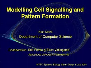
Modelling Cell Signalling Pathways in PEPA. Muffy Calder Department of Computing Science University of Glasgow Jane Hillston and Stephen Gilmore Laboratory for Foundations of Computer Science University of Edinburgh February 2005. Cell Signalling or Signal Transduction *

E N D
Modelling Cell Signalling Pathways in PEPA Muffy CalderDepartment of Computing Science University of GlasgowJane Hillston and Stephen GilmoreLaboratory for Foundations of Computer Science University of EdinburghFebruary 2005
Cell Signalling or Signal Transduction* • fundamental cell processes (growth, division, differentiation, apoptosis) determined by signalling • most signalling via membrane receptors • signalling molecule • receptor • gene effects * movement of signal from outside cell to inside
RKIP Inhibited ERK Pathway MEK Raf-1* RKIP proteins/complexes forward /backward reactions (associations/disassociations) products (disassociations) m1, m2 .. concentrations of proteins k1,k2 ..: rate (performance) coefficients m2 m2 m1 m2 m12 k1/k2 k1 k1 k12/k13 ERK-PP k11 k15 m3 m3 m9 m3 Raf-1*/RKIP m13 k3 K3/k4 k3 k8 m11 RKIP-P/RP MEK-PP/ERK-P m4 m8 Raf-1*/RKIP/ERK-PP k14 k5 k9/k10 k6/k7 m5 m6 m7 m10 MEK-PP ERK RKIP-P RP From paper by Cho, Shim, Kim, Wolkenhauer, McFerran, Kolch, 2003.
RKIP Inhibited ERK Pathway MEK Raf-1* RKIP m2 m2 m1 m2 m12 Pathways have computational content! Producers and consumers. Feedback. k1/k2 k1 k1 k12/k13 ERK-PP k11 k15 m3 m3 m9 m3 Raf-1*/RKIP m13 k3/k4 k3 k3 k8 m11 RKIP-P/RP MEK-PP/ERK-P m4 m8 Raf-1*/RKIP/ERK-PP k14 k5 k9/k10 k6/k7 m5 m6 m7 m10 MEK-PP ERK RKIP-P RP
RKIP Inhibited ERK Pathway MEK Raf-1* RKIP m2 m2 m1 m2 m12 Why not use process algebras for modelling? High level formalisms that make interactions and event rates explicit. k1/k2 k1 k1 k12/k13 ERK-PP k11 k15 m3 m3 m9 m3 Raf-1*/RKIP m13 k3/k4 k3 k3 k8 m11 RKIP-P/RP MEK-PP/ERK-P m4 m8 Raf-1*/RKIP/ERK-PP k14 k5 k9/k10 k6/k7 m5 m6 m7 m10 MEK-PP ERK RKIP-P RP
Process algebra(for dummies) High level descriptions of interaction, communication and synchronisation Eventa Prefixa.P Choice P1 + P2 Synchronisation P1 |l| P2 ¬(ae l) independent concurrent (interleaved) actions ae l synchronised action Constant A = P assign names to components Relations@ (bisimulation) Laws P1 + P2 @ P2 + P1 a a a a a a @ @ b c c b b b c
PEPA Markovian process algebra invented by Jane Hillston with workbench by Stephen Gilmore. PEPA descriptions denote continuous Markov chains. Prefix (a,l).P Choice P1 + P2 competition between components (race) Cooperation/ P1 |l| P1 ¬(a e l) independent concurrent (interleaved) actions Synchronisation a e l shared action, at rate of slowest Constant A = P assign names to components l is a rate, from which a probability is derived - exponential distribution.
Modelling the ERK Pathway in PEPA • Each reaction is modelled by an event, which has a performance coefficient. • Each protein is modelled by a process which synchronises others involved in a reaction. (reagent-centric view) • Each sub-pathway is modelled by a process which synchronises with other sub-pathways. (pathway-centric view)
Signalling Dynamics P2 P1 m2 m1 Reaction Producer(s) Consumer(s) k1react {P2,P1} {P1/P2} k2react {P1/P2} {P2,P1} k3product {P1/P2} {P5} … k1react will be a 3-way synchronisation, k2react will be a 3-way synchronisation, k3product will be a 2-way synchronisation. k1/k2 k4 P1/P2 m3 P5/P6 m4 k3 K6/k7 m6 m5 P6 P5
Reagent View Model whether or not a reagent can participate in a reaction (observable/unobservable): each reagent gives rise to a pair of definitions. P1H = (k1react,k1). P1L P1L = (k2react,k1). P2H P2H = (k1react,k1). P2L P2L = (k2react,k2). P2H + (k4react). P2H P1/P2H = (k2react,k2). P1/P2L + (k3react, k3). P1/P2L P1/P2L = (k1react,k1). P1/P2H P5H = (k6react,k6). P5L + (k4react,k4). P5L P5L = (k3react,k3). P5H +(k7react,k7). P5H P6H = (k6react,k6). P6L P6L = (k7react,k7). P6H P5/P6H = (k7react,k7). P5/P6L P5/P6L = (k6react,k6) . P5/P6H P2 P1 m2 m1 k1/k2 k4 P1/P2 m3 P5/P6 m4 k3 k6/k7 m6 m5 P6 P5
Reagent View Model configuration P1H |k1react,k2react| P2H | k1react,k2react,k4react | P1/P2L |k1react,k2react,k3react| P5L |k3react,k6react,k4react| P6H |k6react,k7react| P5/P6L Assuming initial concentrations of m1,m2,m6. P2 P1 m2 m1 k1/k2 k4 P1/P2 m3 P5/P6 m4 k3 K6/k7 m6 m5 P6 P5
MEK Raf-1* RKIP m2 m2 m1 m2 m12 k1 k1/k2 k1 k12/k13 ERK-PP k11 k15 m3 m3 m9 m3 Raf-1*/RKIP m13 k3 k3/k4 k3 k8 m11 RKIP-P/RP MEK-PP/ERK-P m4 m8 Raf-1*/RKIP/ERK-PP k14 k5 k9/k10 k6/k7 m5 m6 m7 m10 MEK-PP ERK RKIP-P RP Reagent view: Raf-1*H = (k1react,k1). Raf-1*L + (k12react,k12). Raf-1*L Raf-1*L = (k5product,k5). Raf-1*H +(k2react,k2). Raf-1*H + (k13react,k13). Raf-1*H + (k14product,k14). Raf-1*H … (26 equations)
Reagent View model configuration Raf-1*H |k1react,k12react,k13react,k5product,k14product| RKIPH | k1react,k2react,k11product | Raf-1*H/RKIPL |k3react,k4react| Raf-1*/RKIP/ERK-PPL |k3react,k4react,k5product| ERK-PL |k5product,k6react,k7react| RKIP-PL |k9react,k10react| RKIP-PL|k9react,k10react| RKIP-P/RPL|k9react,k10react,k11product| RPH|| MEKL|k12react,k13react,k15product| MEK/Raf-1*L|k14product| MEK-PPH |k8product,k6react,k7react| MEK-PP/ERKL|k8product| MEK-PPH|k8product| ERK-PPH
Pathway View Model chains of behaviour flow. Two pathways, corresponding to initial concentrations: Path10 = (k1react,k1). Path11 Path11 = (k2react).Path10 + (k3product,k3).Path12 Path12 = (k4product,k4).Path10 + (k6react,k6).Path13 Path13 = (k7react,k7).Path12 Path20 = (k6react,k6). Path21 Path21 = (k7react,k6).Path20 Pathway view: model configuration Path10 | k6react,k7react | Path20 (much simpler!) P2 P1 m2 m1 k1/k2 k4 P1/P2 m3 P5/P6 m4 k3 K6/k7 m6 m5 P6 P5
MEK Raf-1* RKIP m2 m2 m1 m2 m12 k1 k1/k2 k1 k12/k13 ERK-PP k11 k15 m3 m3 m9 m3 Raf-1*/RKIP m13 k3 k3/k4 k3 k8 m11 RKIP-P/RP MEK-PP/ERK-P m4 m8 Raf-1*/RKIP/ERK-PP k14 k5 k9/k10 k6/k7 m5 m6 m7 m10 MEK-PP ERK RKIP-P RP Pathway view: Pathway10 = (k9react,k9). Pathway11 Pathway11 = (k11product,k11). Pathway10 + (k10react,k10). Pathway10 … (5 pathways)
Pathway View model configuration Pathway10 |k12react,k13react,k14product| Pathway40 |k3react,k4react,k5product,k6react,k7react,k8product| Pathway30 |k1react,k2react,k3react,k4react,k5product| Pathway20 |k9react,k10react,k11product| Pathway10
What is the difference between the two views/models? • reagent-centric view is a fine grained view • pathway-centric view is a coarse grained view • reagent-centric is easier to derive from data • pathway-centric allows one to build up networks from already known components The two models are equivalent! The equivalence proof, based on bisimulation between steady state solutions, unites two views of the same biochemical pathway.
1 0.041350790041564812 0.0208061151023106323 0.073467759296928994 0.0069353717007701525 0.065161040166416726 0.037375466220971197 0.0113367157494711948 0.0360482059335932869 0.00463984157716770810 0.00569139435096023711 0.0413845661862080312 0.002582808982032050513 0.00480778362079702414 0.0481712379850729615 0.01864067106983505516 0.01674353961951514217 0.0216287435105674518 0.002891255249280381619 0.00497023810042315820 0.0207678071832230221 0.184005485148599922 0.00884605267233758523 0.0141321835645967824 0.003048222164904722425 0.002084470415146022326 0.2047732923318231227 0.0964257689104687428 0.0012831731450123965 1 0.041350790041563532 0.0208061151023106043 0.073467759296924194 0.0069353717007698345 0.065161040166412626 0.037375466220967837 0.0113367157494708898 0.036048205933591569 0.00569139435095978710 0.00463984157716754311 0.0413845661862075212 0.0481712379850750513 0.002582808982031824614 0.0186406710698350415 0.00480778362079673716 0.0167435396195150717 0.02076780718322434518 0.02162874351056822219 0.1840054851486054920 0.00289125524928003821 0.00884605267233746422 0.00497023810042342423 0.01413218356459749924 0.2047732923318296425 0.0964257689104713926 0.003048222164904605327 0.002084470415145398328 0.0012831731450119671 Reagent view Pathway view
What do you do with these two models? -investigate properties of the underlying Markov model. Generate steady-state probability distribution (using linear algebra) and then perform; -Transient analysis e.g. analysis to determine whether a state will be reached. OR -Steady state analysis (more appropriate here) e.g. analysis of the steady state solution. Note: there isn’t one steady state, but a very large “cycle”!
Quantitative Analysis Effect of increasing the rate of k1 on k8product throughput (rate x probability)i.e. effect of binding of RKIP to Raf-1* on ERK-PP. Increasing the rate of binding of RKIP to Raf-1* dampens down the k8product reactions, i.e. it dampens down the ERK pathway.
Quantitative Analysis – by logic Steady state analysis Formula S=? [ERK_PP_H_STATE = 0] PRISM result (after translation):
Quantitative Analysis – by logic Now reduce backward rates (.53) Formula S=? [ERK_PP_H_STATE = 0]
Reagent view and ODEs Activity matrix k1 k2 k3 k4 k5 k6 k7 P1 -1 +1 0 0 0 0 0 P2 -1 +1 0 +1 0 0 0 P1/P2 +1 -1 0 0 0 0 0 P5 0 0 +1 -1 0 -1 +1 P6 0 0 0 0 0 -1 +1 P5/P6 0 0 0 0 0 +1 -1 Column: corresponds to a single reaction. Row: correspond to a reagent; entries indicate whether the concentration is +/- for that reaction. mass action dynamics: dm1 = - k1*m1*m2 + k2*m3 (nonlinear) dt Reagent views tells us producer or consumer. P2 P1 m2 m1 k1/k2 k4 P1/P2 m3 P5/P6 m4 k3 K6/k7 m6 m5 P6 P5
Big Picture abstraction pathway composition Benefits Interactions Relative change Abstraction Behaviour patterns Quantitative analysis stochastic process algebra throughput analysis reagent view pathway view mass action differential equations derive denote Continuous time Markov chains
Bigger Picture abstraction pathway composition Benefits Interactions Relative change Abstraction Behaviour patterns Quantitative analysis experimental data stochastic process algebra throughput analysis reagent view pathway view mass action differential equations derive Matlab multilevel reagent view denote simulate logic PRISM Continuous time Markov chains
Further Challenges • Derivation of the reagent-centric model from experimental data • Quantification of abstraction over networks • zoom in or out • Other dynamics (inhibition) • Functional rates • Very large scale pathways • Model spatial dynamics (vesicles).