Overview of Manufacturing Operations Scheduling: Process and Product-Focused Approaches
This chapter provides an in-depth overview of scheduling in manufacturing operations, focusing on both process and product-focused manufacturing. Learn about job shops, the complexities of scheduling, and the importance of master production schedules (MPS) and material requirements planning (MRP). It also covers key topics like input-output control, Gantt charts, and various sequencing rules such as First-Come, First-Served (FCFS) and Shortest Processing Time (SPT). Understand how world-class companies effectively manage their scheduling to ensure optimal production efficiency.

Overview of Manufacturing Operations Scheduling: Process and Product-Focused Approaches
E N D
Presentation Transcript
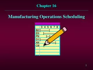
3 4 5 6 7 8 B2 [----------] E5 [-------------- P9 [---] D1 [-------- X8 ----] C6 [- Chapter 16 Manufacturing Operations Scheduling
Overview • Scheduling Process-Focused Manufacturing • Scheduling Product-Focused Manufacturing • Computerized Scheduling Systems • Wrap-Up: What World-Class Companies Do
Scheduling Process-Focused Manufacturing
Process-Focused Manufacturing • Process-focused factories are often called job shops. • A job shop’s work centers are organized around similar types of equipment or operations. • Workers and machines are flexible and can be assigned to and reassigned to many different orders. • Job shops are complex to schedule.
Scheduling and Shop-Floor Decisions Master Production Schedule (MPS) Product Design and Process Plans Material Requirements Plan (MRP) Capacity Requirements Plan (CRP) Order- Processing or Routing Plans Planned Order Releases Report Work Center Loading and Overtime Plan Assignment of Orders to Work Centers Day-to-Day Scheduling and Shop-Floor Decisions
Pre-production Planning • Design the product in customer order • Plan the operations the product must pass through ..... this is the routing plan • Work moves between operations on a move ticket
Common Shop Floor Control Activities • The production control department controls and monitors order progress through the shop. • Assigns priority to orders • Issues dispatching lists • Tracks WIP and keeps systems updated • Controls input-output between work centers • Measures efficiency, utilization, and productivity of shop
Shop Floor Planning and Control • Input-Output Control • Gantt Chart • Finite and Infinite Loading • Forward and Backward Scheduling
Input-Output Control • Input-output control identifies problems such as insufficient or excessive capacity or any issues that prevents the order from being completed on time. • Input-output control report compares planned and actual input, planned and actual output, and planned and actual WIP in each time period
Gantt Charts • Gantt charts are useful tools to coordinate jobs through shop; graphical summary of job status and loading of operations
Gantt Charts Work Centers Wed. Sat. Mon. Tue. Fri. Thu. Machining Fabrication Assembly Test E F G D E F C H C D E D H C Scheduled Progress Setup, Maint.
Assigning Jobs to Work Centers:How Many Jobs/Day/Work Center • Infinite loading • Assigns jobs to work centers without regard to capacity • Unless excessive capacity exists, long queues occur • Finite loading • Uses work center capacity to schedule orders • Popular scheduling approach • Integral part of CRP
Assigning Jobs to Work Centers:Which Job Gets Built First? • Forward scheduling • Jobs are given earliest available time slot in operation • excessive WIP usually results • Backward scheduling • Start with promise date and work backward through operations reviewing lead times to determine when a job has to pass through each operation • Less WIP but must have accurate lead times
Order-Sequencing Problems • Sequencing Rules • Criteria for Evaluating Sequencing Rules • Comparison of Sequencing Rules • Controlling Changeover Costs • Minimizing Total Production Time
Order-Sequencing Problems • We want to determine the sequence in which we will process a group of waiting orders at a work center. • Many different sequencing rules can be followed in setting the priorities among orders. • There are numerous criteria for evaluating the effectiveness of the sequencing rules.
Order-Sequencing Rules • First-Come First-Served (FCFS) Next job to process is the one that arrived first among the waiting jobs • Shortest Processing Time (SPT) Next job to process is the one with the shortest processing time among the waiting jobs • Earliest Due Date (EDD) Next job to process is the one with the earliest due (promised finished) date among the waiting jobs
Order-Sequencing Rules • Least Slack (LS) Next job to process is the one with the least [time to due date minus total remaining processing time] among the waiting jobs • Critical Ratio (CR) Next job to process is the one with the least [time to due date divided by total remaining processing time] among the waiting jobs • Least Changeover Cost (LCC) Sequence the waiting jobs such that total machine changeover cost is minimized
Evaluating the Effectivenessof Sequencing Rules • Average flow time - average amount of time jobs spend in shop • Average number of jobs in system - • Average job lateness - average amount of time job’s completion date exceeds its promised delivery date • Changeover cost - total cost of making machine changeovers for group of jobs
Experience Says: • First-come-first-served • Performs poorly on most evaluation criteria • Does give customers a sense of fair play • Shortest processing time • Performs well on most evaluation criteria • But have to watch out for long-processing-time orders getting continuously pushed back • Critical ratio • Works well on average job lateness criterion • May focus too much on jobs that cannot be completed on time, causing others to be late too.
Example: Sequencing Rules Use the FCFS, SPT, and Critical Ratio rules to sequence the five jobs below. Evaluate the rules on the bases of average flow time, average number of jobs in the system, and average job lateness. JobProcessing TimeTime to Promised Completion A 6 hours 10 hours B 12 16 C 9 8 D 14 14 E 8 7
Example: Sequencing Rules • FCFS Rule A > B > C > D > E Processing Promised Flow JobTimeCompletionTimeLateness A 6 10 6 0 B 12 16 18 2 C 9 8 27 19 D 14 14 41 27 E 8 7 4942 49 141 90
Example: Sequencing Rules • FCFS Rule Performance • Average flow time: 141/5 = 28.2 hours • Average number of jobs in the system: 141/49 = 2.88 jobs • Average job lateness: 90/5 = 18.0 hours
Example: Sequencing Rules • SPT Rule A > E > C > B > D Processing Promised Flow JobTimeCompletionTimeLateness A 6 10 6 0 B 8 7 14 7 C 9 8 23 15 D 12 16 35 19 E 14 14 4935 49 127 76
Example: Sequencing Rules • SPT Rule Performance • Average flow time: 127/5 = 25.4 hours • Average number of jobs in the system: 127/49 = 2.59 jobs • Average job lateness: 76/5 = 15.2 hours
Example: Sequencing Rules • Critical Ratio Rule E > C > D > B > A Processing Promised Flow JobTimeCompletionTimeLateness E (.875) 8 7 8 1 C (.889) 9 8 17 9 D (1.00) 14 14 31 17 B (1.33) 12 16 43 27 A (1.67) 6 10 4939 49 148 93
Example: Sequencing Rules • Critical Ratio Rule Performance • Average flow time: 148/5 = 29.6 hours • Average number of jobs in the system: 148/49 = 3.02 jobs • Average job lateness: 93/5 = 18.6 hours
Example: Sequencing Rules • Comparison of Rule Performance Average Average Average Flow Number of Jobs Job Rule Time in System Lateness FCFS 28.2 2.88 18.0 SPT 25.4 2.59 15.2 CR 29.6 3.02 18.6 SPT rule was superior for all 3 performance criteria.
Controlling Changeover Costs • Changeover costs - costs of changing a processing step in a production system over from one job to another • Changing machine settings • Getting job instructions • Changing material • Changing tools • Usually, jobs should be processed in a sequence that minimizes changeover costs
Controlling Changeover Costs • Job Sequencing Heuristic • First, select the lowest changeover cost among all changeovers (this establishes the first two jobs in the sequence) • The next job to be selected will have the lowest changeover cost among the remaining jobs that follow the previously selected job
Example: Minimizing Changeover Costs Hardtimes Heat Treating Service has 5 jobs waiting to be processed at work center #11. The job-to-job changeover costs are listed below. What should the job sequence be? Jobs That Precede A B C D E A -- 65 80 50 62 B 95 -- 69 67 65 C 92 71 -- 67 75 D 85 105 65 -- 95 E 125 75 95 105 -- Jobs That Follow
Example: Minimizing Changeover Costs • Develop a job sequence: A follows D ($50 is the least c.o. cost) C follows A ($92 is the least following c.o. cost) B follows C ($69 is the least following c.o. cost) E follows B (E is the only remaining job) Job sequence is D – A – C – B – E Total changeover cost = $50 + 92 + 69 + 75 = $286
Minimizing Total Production Time • Sequencing n Jobs through Two Work Centers • When several jobs must be sequenced through two work centers, we may want to select a sequence that must hold for both work centers • Johnson’s rule can be used to find the sequence that minimizes the total production time through both work centers
Johnson’s Rule 1. Select the shortest processing time in either work center 2. If the shortest time is at the first work center, put the job in the first unassigned slot in the schedule. If the shortest time is at the second work center, put the job in the last unassigned slot in the schedule. 3. Eliminate the job assigned in step 2. 4. Repeat steps 1-3, filling the schedule from the front and back, until all jobs have been assigned a slot.
Example: Minimizing Total Production Time It is early Saturday morning and The Finest Detail has five automobiles waiting for detailing service. Each vehicle goes through a thorough exterior wash/wax process and then an interior vacuum/shampoo/polish process. The entire detailing crew must stay until the last vehicle is completed. If the five vehicles are sequenced so that the total processing time is minimized, when can the crew go home. They will start the first vehicle at 7:30 a.m. Time estimates are shown on the next slide.
Example: Minimizing Total Production Time Exterior Interior Job Time (hrs.) Time (hrs.) Cadillac 2.0 2.5 Bentley 2.1 2.4 Lexus 1.9 2.2 Porsche 1.8 1.6 Infiniti 1.5 1.4
Example: Minimizing Total Production Time • Johnson’s Rule Least Work Schedule Time Job Center Slot 1.4 Infiniti Interior 5th 1.6 Porsche Interior 4th 1.9 Lexus Exterior 1st 2.0 Cadillac Exterior 2nd 2.1 Bentley Exterior 3rd
Example: Minimizing Total Production Time 0 1.9 3.9 6.0 7.8 9.3 12.0 L C B P I Idle Exterior Interior Idle L C B P I 0 1.9 4.1 6.6 9.0 10.6 12.0 It will take from 7:30 a.m. until 7:30 p.m. (not allowing for breaks) to complete the five vehicles.
Scheduling Product-Focused Manufacturing
Product-Focused Scheduling • Two general types of product-focused production: • Batch - large batches of several standardized products produced • Continuous - few products produced continuously.... minimal changeovers
Scheduling Decisions • If products are produced in batches on the same production lines: • How large should production lot size be for each product? • When should machine changeovers be scheduled? • If products are produced to a delivery schedule: • At any point in time, how many products should have passed each operation if time deliveries are to be on schedule?
Batch Scheduling EOQ for Production Lot Size • How many units of a single product should be included in each production lot to minimize annual inventory carrying cost and annual machine changeover cost?
Example: EOQ for Production Lots CPC, Inc. produces four standard electronic assemblies on a produce-to-stock basis. The annual demand, setup cost, carrying cost, demand rate, and production rate for each assembly are shown on the next slide. a) What is the economic production lot size for each assembly? b) What percentage of the production lot of power units is being used during its production run? c) For the power unit, how much time will pass between production setups?
Example: EOQ for Production Lots Annual Setup Carry Demand Prod. Demand Cost Cost Rate Rate Power Unit 5,000 $1,200 $6 20 200 Converter 10,000 600 4 40 300 Equalizer 12,000 1,500 10 48 100 Transformer 6,000 400 2 24 50
Example: EOQ for Production Lots • Economic Production Lot Sizes
Example: EOQ for Production Lots • % of Power Units Used During Production d/p = 20/200 = .10 or 10% • Time Between Setups for Power Units EOQ/d = 1,490.7/20 = 74.535 days
Batch Scheduling • Limitations of EOQ Production Lot Size • Uses annual “ballpark” estimates of demand and production rates, not the most current estimates • Not a comprehensive scheduling technique – only considers a single product at a time • Multiple products usually share the same scarce production capacity
Batch Scheduling • Run-Out Method • Attempts to use the total production capacity available to produce just enough of each product so that if all production stops, inventory of each product runs out at the same time
Example: Run-Out Method QuadCycle, Inc. assembles, in batches, four bicycle models on the same assembly line. The production manager must develop an assembly schedule for March. There are 1,000 hours available per month for bicycle assembly work. Using the run-out method and the pertinent data shown on the next slide, develop an assembly schedule for March.
Example: Run-Out Method Assembly March April Inventory Time Forec. Forec. On-Hand Required Demand Demand Bicycle (Units) (Hr/Unit) (Units) (Units) Razer 100 .3 400 400 Splicer 600 .2 900 900 Tracker 500 .6 1,500 1,500 HiLander 200 .1 500 500
Example: Run-Out Method • Convert inventory and forecast into assembly hours Assemb. March March Invent. Time Forec. Invent. Forec. On-Hand Req’d. Dem. On-Hand Dem. Bicycle (Units) (Hr/Unit) (Units) (Hours) (Hours) Razer 100 .3 400 30 120 Splicer 600 .2 900 120 180 Tracker 500 .6 1,500 300 900 HiLander 200 .1 500 20 50 Total 470 1,250 (1) (2) (3) (4) (5) (1) x (2) (2) x (3)