ERROR DRIVEN ACTIVE LEARNING GROWING RADIAL BASIS FUNCTION NETWORK FOR EARLY ROBOT LEARNING
ERROR DRIVEN ACTIVE LEARNING GROWING RADIAL BASIS FUNCTION NETWORK FOR EARLY ROBOT LEARNING. By – Arun Kant Singh. Radial basis function network is expressed as : Where : is vector for system output.

ERROR DRIVEN ACTIVE LEARNING GROWING RADIAL BASIS FUNCTION NETWORK FOR EARLY ROBOT LEARNING
E N D
Presentation Transcript
ERROR DRIVEN ACTIVE LEARNING GROWING RADIAL BASIS FUNCTION NETWORK FOR EARLY ROBOT LEARNING By – Arun Kant Singh.
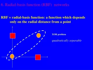
Radial basis function network is expressed as : • Where : is vector for system output. • N0 : is the number of output • X : is the system input • ak : weight vector from the hidden unit ΦK (x) to the output. • µk : kth hidden unit’s center σk : kth hidden unit’s width. • N : Number of radial basis functions Unit.
The growing RBF network starts with no hidden units, and with each learning step, i.e., after the system observes the consequence after an action, the network grows or shrinks when necessary or adjusts the network parameters accordingly. The growth of the network depend on the following conditions : : whether the current network prediction error for the current learning observation is bigger than a threshold. : whether the node to be added is far enough from the existing nodes in the network. : is to check the prediction error within a sliding window to ensure that growth is smooth. Where : x(t) and y(t) are the learning data at tth step. µr (t) : is the center vector of the nearest node to the current input x(t). m : is the length of the observation window.
If the above three conditions are met, then a new node is inserted into the network with the following parameters: aN+1 = e(t) µN+1 = x(t) σN+1 = K||X(t) - µr (t) || where k is the overlap factor between the hidden units. Let Onj be the jth output component of the nth hidden neuron: If rnj < δ for M consecutive learning steps, then the nth node is removed. Where :δ is a threshold.
In ND-EKF, during learning, instead of updating all the network parameters once at each learning step, we update the parameters of each node independently. The parameters of the network are grouped into N0+N components. The first N0 groups are the weights, Wk = [a0k a1k a2k …..aNk ]T;k = 1, 2,….N0 (aij is the weight from ith hidden node to jth output). The other N groups are the parameters of hidden units’ parameters: Wk=[µk T σk] T ; k = 1, 2, ….. N. Hence for kth parameter group at tth learning step, ND-EKF is given by Wk(t) = Wk(t-1) + Kk(t).ek(t) . Where:
Kk(t) is the Kalman gain which is given by : Kk(t) = Pk(t-1).BkT(t) [ Rk(t) + Bk(t).Pk(t-1).BkT(t)]-1 Pk(t) is the error covariance matrix and is updated by Pk(t) = [I – Kk(t).Bk(t)]Pk(t-1) – qI. where : yk(t) : is the kth component of y(t) in training data (x(t); y(t)), Bk(t): is the submatrix of derivatives of network outputs with respect to the kthgroup’s parameters at tthlearning step. Rk(t): is the variance of the measurement noise. q :is a scalar that determines the allowed random step in the direction of the gradient vector. 3. The computational complexity of the node-decoupled EKF is much lower than the global EKF.
In the following, we present the simplified formulae of Kalman gain and error covariance matrix for network weight parameters and hidden unit parameters separately. For the weight parameters : For the weight parameters, Wk = [a0k a1k a2k …..aNk ]T;k = 1, 2,….N0 , as the weights for each output are completely independent of those of other outputs; hence, the system learns the weights for each individual output separately. Therefore we have Bk(t) = [1, Φ1 , Φ2, Φ3 ,…. , ΦN] and the Kalman gain is given by Kk(t ) = Pk(t-1).BkT(t)/( ηk+ λ) Where ηk = Bk(t).Pk(t-1).BkT(t) is a scaler. The error covriancematrics becomes : Pk(t) = [Pk(t-1) –{Pk(t-1). BTk(t).Bk(t)Pk(t-1)/( ηk+ λ)} +qI]
3. For the hidden units : For the parameters of Wk=[µk T σk] T = [µk1 µk1µk1 …. µk1, σk] T, the gradient matrix Bk(t )becomes : Where : In the above x1, x2 , x3 ……xNi are the components of input signal X. 4. The Kalman Filter can be re-written as :
And therefore Pk can be written as : where: and this is a scalar .
To reduce the large mapping error clusters, an error driven active learning approach is presented. Error clustering and Local learning are two key components in active learning. We applied hierarchical error clustering to locate the large error clusters at different levels and used local sub networks to approximate the residual mapping errors of these clusters
Hierarchical error clustering Hierarchical error clustering is used to group the mapping errors simultaneously over a variety of scales by creating a cluster tree. At each step of the hierarchical clustering, only two mapping errors with the nearest distance are joined. The distance between two mapping errors is defined as: Where: ->r and s are two error indexes, ->n is the number of components of each error (location component x, y and error amplitude in our application). ->xri and xsi are error components. ->wi is the weight for the ith component
assign each mapping error to its own cluster and ID. Compute distance between pairs of clusters according to formula . Merge the two clusters that are closest to each other and assign a new ID. Check Count > 1
Once the hierarchical error cluster tree is generated, the robot is driven to move to the areas with large average errors, and capture the data relevant to the learning task . The obtained data is firstly compared with the predicted value from the lower mapping network(s), and then the residual mapping errors are used to train local sub networks. Local sub networks are also built by using growing radial basis function networks trained by SDEKF. Although global growing radial basis function networks, which cover the whole work space, can adjust the number of neurons, and the location and size of each neuron, these adjustments are usually affected by the distribution of the training data If a global network is used in active learning, the active learning data, which is usually from some local areas, will affect the network mapping in other areas.
For a training sample (x(t), y(t)) at time t, the residual error rj for the input of the sub network at the jth layer is computed Where: amli -> is the weights from the ithneuro to the output of the mthsubnetworkwhich covers the current input point x(t) at the lthlayer (l = 0, 1, · · · , j − 1), φmli(x(t)) -> is ith neuron of the mthsubnetwork. Nml ->is the number of the neurons in the mthsubnetwork at the lth layer.
The whole learning system is based on a hierarchical structure of growing radial basis function networks (GRBF). The system firstly uses a GRBF to cover the whole work space. When the mapping error from this network does not change significantly and the map has become saturated. The system triggers the active learning process to build next level of sub-networks if the map becomes saturated. A long-term memory (LTM) stores training data of the most recent trials for later use in the hierarchical error cluster module for analyzing the mapping error distribution. The module “Sig. clusters” selects the large error clusters from the cluster tree generated by the module hierarchical error clustering(HEC).
For each large error cluster, the system generates an active learning position at each learning step, sends this location to the robot and gets information back from the robot’s action. The residual error from previous layers which cover this location is then used to train a local sub-network. Such process continues until the mapping error changes from this cluster cease. The system then conducts the active learning in another area of large error clusters selected by the module HEC and the module “Sig. clusters”. After finishing construction of all the subnetworks in the current layer, the system will continue to generate another level if the mapping error is still large than a threshold.
Error Distribution : Before Active Learining After Active Learining
Mapping error Dendrogram : The horizontal axis is the error cluster index, and the vertical axis is the distance between the two error clusters it links. Big values represent that the two linked clusters are quite different; while small values mean that the two linked clusters are similar.
Mapping Error: The upper curve is the error without active learning while the bottom one is for active learning. The figure only shows the results from the beginning of the active learning and ignores the training of the first layer of the mapping networks.
Comparison between error variances The upper curve is without active learning while the bottom one is for active learning.