Central limit theorem revisited
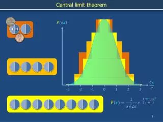
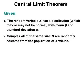
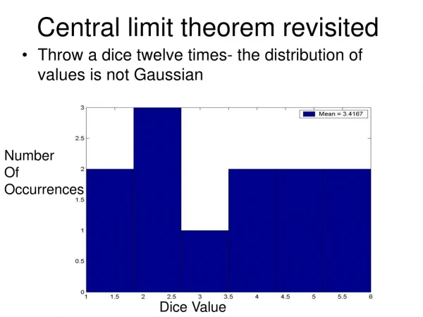
Central limit theorem revisited. Throw a dice twelve times- the distribution of values is not Gaussian. Number Of Occurrences. Dice Value. Repeat twelve dice throws twelve times- find the average for each set of twelve. Number Of Occurrences. Dice Value.


Central limit theorem revisited
E N D
Presentation Transcript
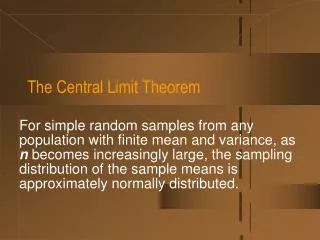
Central limit theorem revisited • Throw a dice twelve times- the distribution of values is not Gaussian Number Of Occurrences Dice Value
Repeat twelve dice throws twelve times- find the average for each set of twelve Number Of Occurrences Dice Value
What is the distribution of the AVERAGE of the 12 sets? Number of Occurrences Mean Dice Value
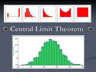
Same as last slide, for 180 sets Number Of Occurrences Average Dice Value of Each set Key Point: Even though the distribution in each set is NOT Gaussian, the average of the sets has a Gaussian Distribution
Time Series 2 Time Series 1 TS2=5*cos(2*t) TS1=cos(2*t) R2 = 1 Perfectly correlated
Time Series 2 Time Series 1 * R2 = 0 No LINEAR correlation TS2=5*cos(2*t) TS1=cos(t)
Time Series 2 Time Series 1 TS2=sin(t) TS1=cos(t) R2 = 0 No correlation
Time Series 2 Time Series 1 TS2=cos(t-pi/4) TS1=cos(t)
Which linear fit minimizes the error in a least squares sense? Hint, what is the fraction of the variance explained implied by each fit? B A C R2= a12 x’2 y’2
Answer C RMS error = .707 implies R2=.5 RMS error = .767
Buying/Selling Nuts and Bolts • Usually when you buy one nut, you buy one bolt as well • Sometimes you miscount a little bit, but most of the time, you go to the store to buy sets of nuts and bolts
If I ask you to go to the store to get 12 nuts and 10 bolts, you trace out 10 units on the bolt axis and 12 units on the bolt axis 10 Bolts 12 NUTS
Alternatively, I could ask for 10 sets of nuts and bolts and 2 extra nuts • Trace 10 units on the nut bolt axis • Trace 2 units on the nut only axis Advantage: We explain more data with a single (rotated) axis
Some additional considerations:Maintaining orthogonality of our axes • Keep the principle axis, make the secondary axis orthogonal to it 11 units On the nut bolt axis -1 unit on the bolt excess axis
Some additional considerations • Rotate the axis about the mean of the data (x and y) • The principle axis is then, the axis which explains the • maximum fraction of the VARIANCE.
In EOF speak • The Empirical Orthogonal Function (also called eigenvector) is the definition of the axes • The Principal Component (also called time series), is the trace of each purchase (data realization) onto the axis
What about buying nuts, bolts, and washers? Number of Nuts
Subtract the mean from each axis Number of Nuts
Define principal axis which explains the most variance It is defined by 1 nut,1 bolt, 2 washers, NORMALIZED
The secondary axis is orthogonal to the primary axis And explains the greatest possibel fraction of the REMAINING variance Number of nuts
The third and final axis is orthogonal to the first two It is therefore uniquely defined by the first two Number of nuts
How do we represent the data that fall on the primary axis? Regress or correlate the each realization of the data against the rotated axis (eigenvector). Data point = [-9 nuts, -9 bolts, -18 washers] Regression onto principle axis= [-9, -9, -18] * [.408, .408, .81] = -22 units The dimensional principal component of the first EOF associated with a normalized axis
Alternatively, we could normalize the PC over all realizations Normalized First PC
Now regress the normalized PCagainst the original nut and bolt data Regression coef. = The number of bolts sold associated with a one standard deviation purchase of the first EOF/PC pair = 6 nuts in this case Alternatively, we could express the PC’s projection onto the bolt data as a correlation =
Repeat the regression with bolts and washers we now the combination of nuts, bolts and washers associated with a standard purchase in the primary EOF/axis [6 NUTS, 6 BOLTS, 12 Washers] if the data was perfect Standard Purchase on The primary axis Multiply by the normalize PC and we have a large percent of our data
Again in EOF speak • The axes definition are the EOFs (Eigenvectors, spatial patterns) • The trace or projection onto the axes for each data realization is the principal component (time series) • Lastly, the fraction of the variance explained along each axis is the eigenvalue or singular value ( will get to this soon)
Some thoughts • 1st EOF answers the question, what linear combination of the data best explains the variance • 2nd EOF answers question, what pattern best explains the REMAINING variance, is severely constrained by orthogonality • Both PCs and EOFs are orthogonal • Direction of EOF is ambiguous to 180 degrees • EOF/PC pairs are uniquely defined by the data set, not the physics!!! • Key Idea: Explain the majority of a large data set with a small number of spatial/temporal patterns
How does this relate to spatial-temporal data At any instance, we represent a spatial pattern by an Nx by Ny matrix representing the data at each grid point We could also think of the data at each time as vector of length Nx * Ny observations let Nx * Ny =M= # of observations at each time
Compose a matrix out of the vector of M observations at each of N observation times. • M = number of observations at each time (Spatial Locations) • N = number of time steps in the data set TIME SPACE Columns refer to a set of M spatial observations at a given time Rows correspond to a time series of observations at a given location
Singular Value Decomposition (SVD)X = USVT Principal Component, time series (normalized) DATA MATRIX Variance Explained by PC/EOF pair EOFs Spatial Structures (Normalized) N M N N M M M N LEADING EOF (Eigenvector) VECTOR LENGTH M (NORMALIZED IN SPACE) Diagonal squared Gives amount Of variance explained First PC/ time series (NORMALIZED in Time)
Eigenvectors, Eigenvalues, PC’s • Eigenvectors explain variance in spatial (observation) dimension; Principle components explain variance in the time (realization of data) dimension. • Each eigenvector has a corresponding principle component. The PAIR define a mode that explains variance. • Each eigenvector/PC pair has an associated eigenvalue which relates to how much of the total variance is explained by that mode.
Fabricated example of spatial temporal data What spatial and temporal patterns most efficiently describe this data set? Are they orthogonal in space? Time?
EOF 1 - 60% variance expl. EOF 2 - 40% variance expl. PC 1 PC 2
Eigenvalue Spectrum EOF 1 - 60% variance expl. EOF 2 - 40% variance expl. PC 1 PC 2 % Variance = Eigenvalue Explained (sum of all Eigenvalues)
Fabricated example of spatial temporal data What spatial and temporal patterns most efficiently describe this data set? Are they orthogonal in space? Time?
EOF 2 PC 1 PC 2
“Data” EOF 1 - 65% variance expl. EOF 2 - 35% variance expl. PC 1 PC 2
This is A composite Not an EOF Cold tongue index
Correlate the cold tongue index time series with SLP at each grid point to get a correlation map
EOF 2: PNA (13% expl.) EOF 1: AO/NAM (23% expl). EOF 3: non-distinct(10% expl.) EOFs of Northern hemisphere sea level Pressure EOFs of Real Data: Winter SLP anomalies Northern Annular mode Arctic Oscillation Pacific North America Mode
EOF 1 (AO/NAM) EOF 2 (PNA) EOF 3 (?) PC1 (AO/NAM) PC2 (PNA) PC3 (?)
PNA - Correlation map (r values of each point with index) PNA – Geopotential Regression map (meters/std deviation of index) Correlation maps vs. regression maps 500 hPa • Correlation maps put each point on ‘equal footing’ • Regression maps show magnitude of typical variability
Regress the PCs of SLP against surface air temperature annomalies The surface air temperature field associated with a one standard deviation NAM or PNA event
Significance • Each EOF / PC pair comes with an associated eigenvalue • The normalized eigenvalues (each eigenvalue divided by the sum of all of the eigenvalues) tells you the percent of variance explained by that EOF / PC pair. • Eigenvalues need to be well separated from each other to be considered distinct modes. First 25 Eigenvalues for DJF SLP Eigenvalue EOF/PC #
These two just barely overlap. Need physical intuition to help judge. Example of overlapping eigenvalues Significance: The North Test First 25 Eigenvalues for DJF SLP • North et al (1982) provide estimate of error in estimating eigenvalues • Requires estimating degrees of freedom (DOF) of the data set. • If eigenvalues overlap, those EOFs cannot be considered distinct. Any linear combination of overlapping EOFs is an equally viable structure. Eigenvalue EOF/PC #
Validity of PCA modes: Questions to ask • Is the variance explained more than expected for null hypothesis (red noise, white noise, etc.)? • Do we have an a priori reason for expecting this structure? Does it fit with a physical theory? • Are the EOF’s sensitive to choice of spatial domain? • Are the EOF’s sensitive to choice of sample? If data set is subdivided (in time), do you still get the same EOF’s?
Practical Considerations • EOFs are easy to calculate, difficult to interpret. There are no hard and fast rules, physical intuition is a must. • Due to the constraint of orthogonality, EOFs tend to create wave-like structures, even in data sets of pure noise. So pretty… so suggestive… so meaningless. Beware of this.
Practical Considerations • EOF’s are created using linear methods, so they only capture linear relationships. • By nature, EOF’s give are fixed spatial patterns which only vary in strength and in sign. E.g., the ‘positive’ phase of an EOF looks exactly like the negative phase, just with its sign changed. Many phenomena in the climate system don’t exhibit this kind of symmetry, so EOF’s can’t resolve them properly.
Regression of Arctic oscillation on zonal wind annomalies and temperature Zonal Wind Pressure Z Y m/s