Download
1 / 30
310 likes | 586 Vues
A Soil-water Balance and Continuous Streamflow Simulation Model that Uses Spatial Data from a Geographic Information System (GIS). Advisor: Dr. David Maidment Research Sponsor: Hydrologic Engineering Center. Overview. Hydrology review: Event-based vs. continuous simulation models

E N D
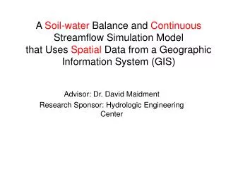
A Soil-water Balance and Continuous Streamflow Simulation Modelthat Uses Spatial Data from a Geographic Information System (GIS) Advisor: Dr. David Maidment Research Sponsor: Hydrologic Engineering Center
Overview • Hydrology review: Event-based vs. continuous simulation models • Research objective • Study area • Spatial Data • radar precipitation, USDA soils • spatial analysis, parameter estimation • information transfer from GIS to an external model • Hydrologic process representation • Summary
Hydrologic Simulation HMS Basin Schematic SHOW SLIDE WITH LOSS RATES ETC.!! EVENT SIMULATION Well-known computer programs: HEC-1, HMS, TR-20 Sub-basin hydrograph methods: • Loss rate • Transform • Baseflow recession
Hydrologic Simulation(cont.) CONTINUOUS SIMULATION evaporation rainfall • Well known computer • programs: • USGS PRMS/Stanford • NWS/Sacramento • HEC Continuous Simulation Model interception and depression storage surface runoff soil root zone soil transmission zone groundwater storage zone(s) subsurface runoff leakage
Continuous • more physical processes represented • antecedent storm conditions are known • complex -- many more parameters • Event • simple • infiltration losses are a sink • difficult to initialize PROS & CONS APPLICATIONS Continuous Event hydrologic/hydraulic design flood forecasting real time water control water resources planning climate change impacts on streamflow Event vs. Continuous Simulation Neither model provides mass closure for the entire hydrologic cycle.
Research Objectives • Develop and test a practical model that uses data describing spatial variability of soils and rainfall • - Develop GIS/hydrology procedures applicable anywhere in the U.S. • - Does added information improve runoff estimates? -- Particularly with regard to the validation stage. • Make results reproducible by automating and working from standard databases. • What spatial scales and modeling complexity are practical and useful?
Study Area • Little Washita River Watershed • 600 km2 • Climate: moist and subhumid • Why choose Little Washita? • NWS NEXRAD Stage III rainfall data • Higher resolution soils data than is generally available. • Site of numerous hydrologic and remote sensing studies -- data available for calibration and validation.
Problem Description climate station streamflow gage
NEXRAD Precipitation Data • Stage III Product • 4 km x 4 km grid • hourly estimates • Composite of information from 17 radars and 500 rain gages
Density of Precipitation Gages • 114 Oklahoma Climate • Stations (Density ~ 1 gage/ 1600 km2) • 100 NEXRAD Cells Per Gage
USDA STATSGO Soils Data Mapunit OK002 Map unit: grouping of map components. Components: typically identify soils with similar properties.
Spatial Variability in Soils • Polygon 1: Mapunit OK151 • 89 % Sandy loam • 6% Loam • 2% Silty clay loam • 2% Clay • 1% Loamy sand • Polygon 2: Mapunit OK103 • 56 % Loam • 30% Silt Loam • 14% Sandy loam Polygon 2 only comprises 10% of all polygons in mapunit OK103. STATSGO County Level Data 2 1
1. Calculate soil component properties using attribute tables and lookup table Component properties dBase file 2. Intersect the precipitation cells with the watershed boundary 3. Determine the component names and component percentages in each NEXRAD cell. NEXRAD cell/watershed shape file 4. Determine the average flowlength from each NEXRAD cell the watershed outlet. Main GIS Procedures • Assumed inputs: • Coverage of Modeling Units (I.e. NEXRAD Cells, Thiessen polygons) • Watershed boundaries • Flowlength grid • STATSGO/SSURGO coverage w/ component and layer tables
Texture Name to Soil Parameters 12 standard USDA classes 719 STATSGO texture names Soil parameters
GIS as a Pre-processor for Hydrologic Models • + Add spatial information • + Automate/Create a Reproducible Product • - Increase computational burden Accounting for spatial variability in a simple way increases the computational burden in the Little Washita by a factor of : 55 cells * 10 components/cell = 550 LESSON: KEEP MODEL SIMPLE
Soil-water Balance Model evaporation infiltration direct runoff root zone transmission zone percolation GW Reservoir(s) subsurface runoff
Actual profile Idealized profile qi qo q qi q qo r r L soil depth soil depth Dq f Green-Ampt Infiltration Model
Initial Eff. Saturation = 0.7 Direct Runoff = 5.1 cm Infiltration Rate as a Function of InitialMoisture Content Infiltration and Precipitation Rates vs. Time for a Loam Soil 7 Initial Eff. Saturation = 0.2 Direct Runoff = 3.5 cm 6 5 4 Rate (cm/hour) 3 2 1 0 1 2 3 4 5 6 7 8 9 10 11 time (hours)
Percolation/Redistribution t = 1 t = 2 t = 3 t = 1 t = 2 t = 3 qi qo qi qo Layer 1 soil depth Layer 2
Evaporation • Evaporation depends on many factors including : • energy available at the surface • water content of the soils • soil type • vegetation characteristics • atmospheric conditions
1 function, f(q) moisture extraction 0 q q q fc wp c soil moisture fraction Evaporation E = f(q)*PE • Seasonal effects? • PE changes as soil dries out. • Penman-Monteith is widely cited alternative but how do you determine surface resistance, especially when the soil begins to dry out?
ARM Data Streams • EBBR : Energy Budget Bowen Ratio • SWATS : Soil Water and Temperature Systems • SMOS : Surface Meteorological Observation Stations Questions and Data Related to Evaporation How to account for the following factors using a simple (daily) model? • How to quantify influence of the moisture state • on the evaporation rate. • To what depth(s) does surface drying influence soil • moisture ? • Is it possible to account for seasonal effects?
Bowen Ratio Method Lo Si aSi Li Rn = Si(1-a) + Li-Lo Rn + H + lE + G = 0
SWATS Data - heat dissipation sensors calibrated against matric potential - water retention curve used to estimate soil water - measurements at eight depths
Summary • Utilize spatial data describing soils and rainfall in a hydrology model. • GIS programs are used to automate parameter estimation. • Evaluate soil-water balance model using both observed soil moisture and runoff data. • Data availability determines model complexity.