2D Collimator Analysis
2D Collimator Analysis. Indirect coupled field analysis. Technique. Previous analysis has involved direct coupled fields ANSYS solves the thermal and structural components for each time step as 1 analysis.


2D Collimator Analysis
E N D
Presentation Transcript
2D Collimator Analysis Indirect coupled field analysis
Technique • Previous analysis has involved direct coupled fields • ANSYS solves the thermal and structural components for each time step as 1 analysis. • The indirect method solves the thermal and structural components separately for each time step. • For short time intervals a constant temperature can be assumed, which saves on analysis time.
2D Data Luis gave me several files giving heat deposition values for beam strikes at positions 2mm and 10 mm from the top of a graphite-titanium collimator for 250 GeV and 500 GeV beams. I rearranged the data into a form acceptable for ANSYS and used data from the Y-Z plane, at x=0. This should give the worst case scenario being directly in the path of the beam. Initially I used data from a 250GeV beam 2mm from the top. Approximate line of 250GeV beam
Heat deposition pattern at x=0 This is a matlab produced figure showing the heat deposition. There is a lot of distortion in the figure. The aspect ratio is 300:1. Unfortunately I couldn’t create a key explaining what heat load the temperatures relate to, other than red is the maximum and blue is the minimum. 6.45mm<y<6.55mm -15mm<z<15mm
Initial model • I created a 2D model measuring from 6.45mm to 6.55mm in Y, and -15mm to 15mm in Z. • For simplicity I neglected the graphite and assumed the model was made entirely of Ti-6Al-4V. • I used the data used to create the figure shown in slide 4. • I applied the heat load for 1 picosecond split into 10 smaller steps. I took the temperature rise from the 10th step and used this in a static structural analysis.
Temperature distribution After 1ps of heating ANSYS predicted the maximum temperature to be 283.43°C The distortion in Y-Z is slightly different to that shown on slide 4. The figure also appears to be smoother. This is because ANSYS has interpolated values between the nodes.
Stress in Z through material The model was fixed in the z direction. Theoretically with a TEC of 9.2x10⁻⁶m°-1 and ΔT= 283.43°C there should be an expansion of .0026m per metre if the model was free to move. But as the material is constrained by boundary condition this leads to a strain of -0.26%. The bottom edge of the area was fixed so it couldn’t move in either direction, set to plane stress so the model was free to move into and out of plane By multiplying the strain by the Young’s Modulus the stress can be calculated. This works out to be -295.88MPa. This agrees with the result from ANSYS.
Transient Analysis I took the temperature figures and applied them to a structural model in two stages. The first stage ramped linearly from 0°C to the maximum temperature in 1ps with 10 sub steps. The second stage applied the maximum temperature constantly for 10ns. A subsequent test showed that the maximum temperature would decrease by 0.045°C after 10ns.
SY at 1ps The model is constrained in z by the boundary condition, but it is free to move in x because its set to plane stress. The inertia of the unheated area causes the model to effectively be constrained in y. The stress in y and z is predicted by this equation: This gives a value of -423MPa. This agrees with the ANSYS result.
Model • Now we have a basic model working and understand what is going on we’ll try using more complicated geometry. • 2D symmetric collimator made from Titanium. Due to some confusion with coordinate systems this model has a lower profile than intended. A mesh size of 50microns was used. This is 5 times larger than the ideal size, but ANSYS wouldn’t allow a 10micron mesh. This caused some problems, one of which being a non-uniform distribution of nodes along the beam path. ANSYS interpolates the heat load to the nearest node which led to a strange heating pattern through the material. This is an artefact of the meshing.
Heat data was taken from a previous Fluka run by Luis. • This was for an asymmetric graphite and titanium collimator.
Reflected Wave Heated zone Wave interaction Graph of stress along reflected wave The peaks are at the interaction point