Sub Exponential Randomize Algorithm for Linear Programming
This presentation by Oz Lavee explores an innovative sub-exponential randomized algorithm for solving linear programming (LP) problems, highlighting significant advancements over traditional exponential algorithms. Leveraging a combination of Clarkson's methods and sub-exponential bounds, the algorithm efficiently addresses LP issues with n inequalities and d variables in expected time. The basics of linear programming are defined, including dimensions, constraints, and key algorithms involved. This approach demonstrates improved computational efficiency and provides insights into basis selection and constraint violations.

Sub Exponential Randomize Algorithm for Linear Programming
E N D
Presentation Transcript
Sub Exponential Randomize Algorithm for Linear Programming Paper by: Bernd Gärtner and Emo Welzl Presentation by : Oz Lavee
Linear programming • The linear programming problem is a well known problem in computational geometry • The last decade brought a progress in the efficiency of the linear programming algorithms • Most of the algorithms were exponential in the dimension of the problem
Linear programming • The last progress is a randomized algorithm that solve linear programming problem with n inequalities and d variables (Rd ) in expected time of: This algorithm that we will see is a combination of Matoušek and Kalai sub exponential bounds and Clarkson algorithms
Definition : Linear programming problem • Find a non negative vector x Rd that minimize cTx subject to n linear inequalities Ax b where x 0 • C – d-vector represent direction • X – d-vector • A[n,d] – n inequalities over d variables
Example over R2 h1 X h2 C h1,h2 - inequalities
Definitions • let H be the set of n half spaces defined by Ax b • Let H+be the set of d halfspaces defined by X0 • For a G H H+we definevG as the lexicographically minimal point x minimizing • cTx over hG h
Definitions : basis • A set of halfspacesBH H+is called a basis • if ,.vB is finite and for any subsetB’ of B • vB’<vB • A basis of G is a minimal subset B G such that • vB = vG
Definitions : violations • a constraint h H H+is violated by G if and only if vG < vG {h} • h is violated by vG ifh is violated by G G= {h1,h3} h = h2 h1 h2 vG h3
Definitions : extreme • a constraint h Gis extreme in G if vG-{h} < vG h1 G = {h1,h2,h3} h2 is extreme vG h2 h3
Lemma 1 1. For F G H H+, vF < vG 2. vF,vGare finite andvF = vG . h is violated by F if and only if h is violated by G. 3. If vG is finite then any basis of G has exactly d constraints , and G has at the most d extreme constraints
The algorithm • Our algorithm is a combination of 3 algorithms that use each other: 1. Clarkson first algorithm (CL1) for n>>d 2. Clarkson second algorithm (CL2) for 3. Subexponenial algorithm(subex) for 6d2 CL1 n>>d CL2 subex 6d2
Clarkson First Algorithm (CL1) • set H of n constraints where n>>d • We choose a random sample R H of size ,compute vR and the set V of constraints from H that are violated by vR • If V is not too large we add it to initially set G = H+ , choose another sample R and compute VR G and so on…
Clarkson First Algorithm (CL1) • CL1 (H) if n < 9d2 then return CL2(H) else r = , G = H+ repeat choose random v = CL2 (R) V = {h H | v violate h} if then G = GV until V = Ø return v
Two important facts Fact 1: • The expected size of V is no more than • The probability that |V| > is at the most The number of attempts to get a small enough V expected to be at the most 2
Three important fact Fact 2: • If any constraint is violated by v = vGR then for any basis B of H there must be a constraint that is violated by v. • The number of expansion of G is at the most d
CL1 Run time • CL1 compute vH H+ with expected o(d2n) operations and at the most 2d calls to CL2 with constraints
Clarkson Second Algorithm CL2 • This algorithm is very similar to the CL1 with the main different that instead of forcing V to be in the next iteration We increase the probability of the elements in v to be chosen for R in the next iteration
Clarkson Second Algorithm CL2 • We will use factor µ for each constraint that will be initialized to 1 . • For any constraint in V we will double his factor • For any basis B the elements of B increase so quickly that after a logarithmic time they will be chosen with high probability
Clarkson Second Algorithm CL2 • CL2 (H) if n 6d2 then return subex(H) else r = 6d2 repeat choose random v = subex (R) V = {h H | v violate h} if then for all h V do µh = 2µh until V = Ø return v
Lemma 4 • Let k be a positive integer then after kd Successful Iterations we have For any basis B of H
Run time CL2 • Since and since 2 > e1/3 after big enough k 2k > nek/3 • let k = 3ln(n) 2 k = n3ln2 > n2 = ne3ln(n)/3 • There will be at the most 3dln(n) successful iterations • There will be at the most 6dln(n) iterations
Run time CL2 • In each iteration there are O(dn) arithmetic operations and one call to subex • Totally O(d2nlogn) operations and 6dln(n) calls to subex
The Sub Exponential Algorithm (SUBEX) • The idea : • H a group of n constraints . • Remove a random constraint h • Compute recursively vH-{h} • If h is not violated then done. • Else try again by removing (hopefully different) constraint • The probability that h is violated is d/n
The Subex Algorithm • In order to get efficiency we will pass to the subex procedure in addition to the set G of constraints a candidate basis • We assume that we have the following primitive procedures: • Basis(B,h) : calculate the basis of B {h} • Violation test • Calculate VB of basis B
The Subex Algorithm Subex(G,B) if G=B return (VB,B) else choose random hG-B (v,B’) = Subex(G- {h},B) if h violates v return Subex(G,basis(B’,h)) else return (v,B’)
The Subex Algorithm • The number of steps is finite since: • The first recursive call decrease the number of constraints • The second recursive call increase the value of the temporal solution • Inductively it can be shown that the step keeps the correctness of the temporal solution
The Subex Algorithm Run Time • The subex algorithm is computing vH H+ with • We called the subex algorithm with 6d2 constraints so the run time for each call to subex is
Total Run Time • The runtime of cl2 = O(d2nlogn + 6dln(n)Tsubex(6d2) = • The runtime of cl1 =
The Abstract Framework • We can expand this algorithm to be used on larger range of problems. • Let H be a finite set • let (W{-},) linear ordered set of values • Let w : 2H W{-} value function
The Abstract Framework • Our goal : to find a minimal subset BH where w(B) = w(H) • We can use the algorithm that we saw in order to solve this problem if 2 axiom are satisfied.
The axioms • For any F ,G such that FG H we have w(F)w(G) .(monotonicity) • For any FG H with w(F) = w(G) if hH w(G) < w(G {h}) than w(F) < w(F {h})
LP-type problems • If those axioms hold for a definition of a problem we will call it LP-type problem • From lemma 1 we can see that the linear programming problem is LP-type.
LP-type problems • For the efficiency of the algorithm we need one more parameter for (H,w): the maximum size of any basis of H which is referred to as the combinatorial dimension of (H,w) denote as
LP-type problems • Any LP-type problem can be solved using the above algorithm but it is not necessarily be in sub exponential time • In order to have sub exponential time the problem should have the property of basis regularity • Basis regularity – all the basis has exactly constraints
LP-type problems - Examples • Smallest closing ball- given a set of n points in Rd find the smallest closing ball (combinatorial dimension- d+1) • Polytope distance – given two polytopes P,Q. compute pP q Q minimizing dist (p,q) (combinatorial dimension- d+2)
Summery • We have seen a randomized sub exponential in d-space algorithm for the linear programming problem • We have seen the family of LP-type problems
References • Linear-programming – Randomization and abstract frame work / Bernd Gärtner and Emo welzl