The Normal distributions
The Normal distributions. BPS chapter 3. © 2006 W.H. Freeman and Company. Objectives (BPS 3). The Normal distributions Density curves Normal distributions The 68-95-99.7 rule The standard Normal distribution Using the calculator to find Normal proportions

The Normal distributions
E N D
Presentation Transcript
The Normal distributions BPS chapter 3 © 2006 W.H. Freeman and Company
Objectives (BPS 3) The Normal distributions • Density curves • Normal distributions • The 68-95-99.7 rule • The standard Normal distribution • Using the calculator to find Normal proportions • Finding a value given a proportion
Density curves A density curve is a mathematical model of a distribution. It is always on or above the horizontal axis. The total area under the curve, by definition, is equal to 1, or 100%. The area under the curve for a range of values is the proportion of all observations for that range. From: Relative area enclosed by bars of histogram To: Relative area under density curve.
Density curves come in any imaginable shape. Some are well-known mathematically and others aren’t.
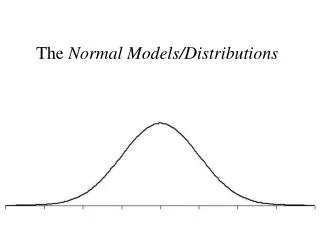
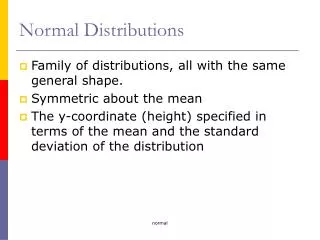
Normal distributions Normal—or Gaussian—distributions are a family of symmetrical, bell- shaped density curves defined by a mean m (mu) and a standard deviation s (sigma): N (m, s). x x e = 2.71828… The base of the natural logarithm π = pi = 3.14159…
Normal distributions Normal—or Gaussian—distributions are a family of symmetrical, bell- shaped density curves defined by a mean m (mu) and a standard deviation s (sigma): N (m, s). Note: we use m and s instead of xBar and s to emphasize that the normal density is an idealized theoretical model of the actual distribution. x x e = 2.71828… The base of the natural logarithm π = pi = 3.14159…
Assume Same Scale on Horizontal and Vertical (not drawn) Axes. The normal density curve! Shape? Center? Spread? Area Under Curve? How does the standard deviation affect the shape of the normal density curve? How does the magnitude of the standard deviation affect a density curve?
Here the means are different (m = 10, 15, and 20) while the standard deviations are the same (s = 3). A family of density curves Here the means are the same (m = 15) while the standard deviations are different (s = 2, 4, and 6).
All Normal curves N (m, s) share the same properties (page 71) Heights of Young Women • About 68% of all observations are within 1 standard deviation (s) of the mean (m). • About 95% of all observations are within 2 s of the mean m. • Almost all (99.7%) observations are within 3 s of the mean. • This is called the 68-95-99.7 Rule (aka Empirical Rule) • Let’s work Problem 3.6 on Page 74 Inflection point mean µ = 64.5 standard deviation s = 2.5 N(µ, s) = N(64.5, 2.5) Reminder: µ (mu) is the mean of the idealized curve, while is the mean of a sample. σ (sigma) is the standard deviation of the idealized curve, while s is the s.d. of a sample.
How to quickly sketch a normal distribution • The empirical rule says that 99.7% of the population lies between m – 3s and m + 3s. • This means that there is very little data outside this range. • Thus the normal density curve is almost identical with the x-axis outside the interval from m – 3s to m + 3s. • So the “visible part” of the bell-shaped density curve is between m – 3s and m + 3s. • Example: sketch the N(m = 100, s = 15) distribution.
My shorthand notation for normal distributions • I abbreviate the statement “X is normal with mean m = 64.5 and standard deviation s = 2.5” as follows: • …sometimes I’ll leave off the m and s: X ~ N(m = 64.5, s = 2.5) X ~ N(64.5, 2.5)
Standardizing: How many standard deviations from the mean height is the height of a woman who is 68 inches? Who is 58 inches? Density Curve for X ~ N(m = 64.5, s = 2.5) X = height (in)
Standardizing: How many standard deviations from the mean height is the height of a woman who is 68 inches? Who is 58 inches? Density Curve for X ~ N(m = 64.5, s = 2.5) X = height (in) Z = num. s. d.
Standardizing: How many standard deviations from the mean height is the height of a woman who is 68 inches? Who is 58 inches? Density Curve for X ~ N(m = 0, s = 1) Z = num. s. d.
Standardizing: How many standard deviations from the mean height is the height of a woman who is 68 inches? Who is 58 inches? Density Curve for X ~ N(m = 0, s = 1) Z = num. s. d. The Standard Normal Distribution (m = 0, s = 1)
Standardizing: Standard Normal Distribution Because all Normal distributions share the same properties, we can standardize our data to transform any Normal curve N (m, s) into the standard Normal curve N (0,1). N(64.5, 2.5) N(0,1) => Standardized height (no units) For each x we calculate a new value, z (called a z-score). The z-score is the number of standard deviations that a data value x is from the mean.
Standardizing: calculating z-scores A z-score measures the number of standard deviations that a data value x is from the mean m. Using the previous slides, find the z-score of a woman whose height is 58 inches; whose height is 73 inches. • When x is larger than the mean, z is positive. • When x is smaller than the mean, z is negative. • If x has a normal distribution with mean m and standard deviation s , then z will have a standard normal distribution.
Standardizing: converting z-scores back to the original units Now let’s go backwards. Given a z-score find the corresponding data value x. How? Solve the equation for x We get For the height data on the previous slides, how tall is a woman whose z-score is z = 1.7?
Example: X = Women’s heights N(µ, s) = N(64.5, 2.5) Women’s heights follow the N(64.5″,2.5″) distribution. Using the empirical rule, determine what percent of women are shorter than 67 inches tall (that’s 5′7″)? Area= ??? Area = ??? mean µ = 64.5" standard deviation s = 2.5" x (height) = 67" m = 64.5″ x = 67″ z = 0 z = 1 We calculate z, the standardized value of x: Because of the 68-95-99.7 rule, we can conclude that the percent of women shorter than 67″ should be, approximately, .68 + half of (1 − .68) = .84, or 84%.
Using Our Calculators to Find the Percent of Women Shorter than 67” • TI-83 Calculator Command: Distr|normalcdf • Syntax: normalcdf(left, right, mu, sigma) = area under normal curve (with mean mu and standard deviation sigma)from left to right • mu defaults to 0, sigma defaults to 1 • Infinity is 1E99 (use the EE key), Minus Infinity is -1E99 Normalcdf(-1E99, 67, 64.5, 2.5) Can we compute using z-scores?? N(µ, s) = N(64.5”, 2.5”) Normalcdf(-1E99,1,0,1)=Normalcdf(-1E99,1) Area ≈ 0.84 Question:What percent of women are taller than 67“?? Area ≈ 0.16 m = 64.5” x = 67” z = 1
My “P” notation for proportions • I abbreviate the statement “the proportion of the population with X between 65 and 70” as follows: • …for a normal distribution, there is no difference between this and P(65 < X < 70) P(65 <=X<= 70) (Why?)
Draw Picture Compute State Answer Normalcdf(820,1E99,1026,209) Normalcdf(-.99,1E99) Area right of 820 = Total area − Area left of 820 = 1 − 0.1611 ≈ 84% Answer: Approximately 84% of students who took the SAT in 2003 scored at least 820. Note: The actual data may contain students who scored exactly 820 on the SAT. However, the proportion of scores exactly equal to 820 being 0 for a normal distribution is a consequence of the idealized smoothing of density curves. The National Collegiate Athletic Association (NCAA) requires Division I athletes to score at least 820 on the combined math and verbal SAT exam to compete in their first college year. The SAT scores of 2003 were approximately normal with mean 1026 and standard deviation 209. What proportion of all students would be NCAA qualifiers? P(X ≥ 820)
Draw Picture Compute State Answer Normalcdf(720,820,209) Normalcdf(-1.46,-0.99) About 9% of all students who take the SAT have scores between 720 and 820. The NCAA defines a “partial qualifier” eligible to practice and receive an athletic scholarship, but not to compete, as a combined SAT score of at least 720. What proportion of all students who take the SAT would be partial qualifiers? P(720 <= X<=820)
One cool thing about working with normally distributed data is that we can manipulate it and then find answers to questions that involve comparing seemingly non-comparable distributions. We do this by “standardizing” the data. All this involves is changing the scale so that the mean now equals 0 and the standard deviation equals 1. If you do this to different distributions, it makes them comparable. N(0,1)
Example: comparing test scores • Andrew and Brian are in two different math classes. • Andrew scored 114 out of 120 on his exam. The class average was 96, with a standard deviation of 12. • Brian scored 162 out of 180 on his exam. His class average was 126, with a standard deviation of 22. • The distributions of exam scores were normal for both classes. • Who did better, Andrew or Brian? • In terms of raw scores… • In terms of z-scores… • In terms of cumulative proportions…
Finding a value given a proportion When you know the proportion, but you don’t know the x-value that represents the cut-off, you have the inverse problem. • State the problem and draw a picture. • 2. Use the invNorm key to find the corresponding x or z. • Syntax: • invNorm(area,mu,sigma)=x • x is a value of the quantitative variable • area is the area to the left of x under normal curve with mean mu and standard deviation sigma.
Area = 0.75 64.5 X = ??? Example: X = Women’s heights Women’s heights follow the N(64.5″,2.5″) distribution. What is the 75th percentile for women’s heights? Draw a picture! • Compute: • We will use our calculator to get X mean µ = 64.5" standard deviation s = 2.5" proportion = area under curve=0.75 Calculator command: invNorm(0.75, 64.5, 2.5) State Answer: The 75th percentile for women’s heights is X = 66.19”, or 5’ 6.19”.