Download
1 / 19
190 likes | 210 Vues
This research outlines the comparison between fixed window and slide window methods in calibrating cosmic data, focusing on signal extraction and parameter evaluation. The study delves into conversion factors, calibration comments, and discrepancy analysis, shedding light on the challenges in data analysis and calibration techniques. The findings prompt further investigation to understand the underlying reasons for calibration issues and data discrepancies.

E N D
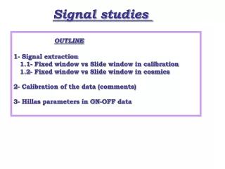
Signal studies OUTLINE 1- Signal extraction 1.1- Fixed window vs Slide window in calibration 1.2- Fixed window vs Slide window in cosmics 2- Calibration of the data (comments) 3- Hillas parameters in ON-OFF data
1.1- Fixed window vs Slide window in calibration Fitted Charge inner pixels Slide window (6 slides) Fixed window (3-10 slide) David Paneque, MPI Muenchen
1.1- Fixed window vs Slide window in calibration Fitted Charge Outer pixels Slide window (6 slides) Fixed window (3-10 slide) David Paneque, MPI Muenchen
1.1- Fixed window vs Slide window in calibration RMS pedestal Inner pixels Slide window (6 slides) Fixed window (3-10 slide) David Paneque, MPI Muenchen
1.1- Fixed window vs Slide window in calibration RMS pedestal Outer pixels Slide window (6 slides) Fixed window (3-10 slide) David Paneque, MPI Muenchen
1.1- Fixed window vs Slide window in calibration Reduced / <Q> for inner pixels Slide window (6 slides) Fixed window (3-10 slide) Mean = 0.240 Sigma = 0.018 Mean = 0.235 Sigma = 0.017 <Nphe> = (<Q> / )2 x F2 = 23 ph. David Paneque, MPI Muenchen
1.1- Fixed window vs Slide window in calibration Reduced / <Q> for outer pixels Slide window (6 slides) Fixed window (3-10 slide) Mean = 0.152 Sigma = 0.016 Mean = 0.140 Sigma = 0.017 <Nphe> = (<Q> / )2 x F2 = 63 ph. David Paneque, MPI Muenchen
1.1- Fixed window vs Slide window in calibration Conversion factors for inner pixels Slide window (6 slides) Fixed window (3-10 slide) David Paneque, MPI Muenchen
1.1- Fixed window vs Slide window in calibration Conversion factors for inner pixels Slide window (6 slides) Fixed window (3-10 slide) David Paneque, MPI Muenchen
Maxim and Hendrik studied the arrival times of pulses from Cosmics in the FADC slices. Pulses DO arrive quite late Fixed window misses part of the signal This explains PARTLY discrepancy between Berlin’s signal (200 phe) and Munich signal (350 phe) 1.2- Fixed window vs Slide window in cosmics Slide window produces a SIZE about 30-40 % higher than Fixed window (3-10 slide) -->> See Munich group web page David Paneque, MPI Muenchen
1.2- Comments on the calibration of the data Inspection of the calibration runs before calibrating data (MANUALLY) David Paneque, MPI Muenchen
CONVERSION FACTORS for all calibration runs taken In Crab Feb 15th observations David Paneque, MPI Muenchen
Inspection of individual conversion factors evolution Fitted charge vs Calibration run for pixel 200 (Crab Feb 15th) David Paneque, MPI Muenchen
Inspection of individual conversion factors evolution Fitted charge vs Calibration run for pixel 200 (Crab Feb 15th) David Paneque, MPI Muenchen
Mean = 0.140 Sigma = 0.017 Mean = 0.235 Sigma = 0.017 63 ph. 23 ph. Rejection (Set conversion factor to ZERO) of those pixels with “strange” behaviour <Q> < 50 ADC counts Reduced /<Q> away by more than 4 sigmas of the distribution (inner/outer)
Rejection (Set conversion factor to ZERO) of those pixels with “strange” behaviour David Paneque, MPI Muenchen
1.2- Comments on the calibration of the data Inspection of the calibration runs before calibrating data (MANUALLY) • Rejection of calibration runs in order to not destroy data • Usage of “closest” calibration run to calibrate a given data run (regardless of ON-OFF) in order to correct for drifts in PMT response (PMT HV ??) • Rejection of those pixels with “strange” behaviour This procedure can OBVIOUSLY be improved. It has been just a first approach to the be able to analyze data “in a decent way”… David Paneque, MPI Muenchen
THIS IS JUST A TEMPORAL SOLUTION. STILL A LOT OF WORK TO BE DONE TO UNDERSTAND REASONS FOR THESE DEFFICIENCIES What is the reason for “corrupted” calibration runs, conversion factors drifts, “strange pixels” ?? Problem with PMT HV ? DAQ/FADC Problem ? In my opinion, a group of people should take the responsibility of checking IN DETAIL (Runs, pixels, events) calibration data, and later cosmic data, in order to understand and correct ALL the problems in the pixel chain. Why OUTER pixels have a conversion factor of only 2.7 Times larger than INNER pixels ? Why do they have such a “wide” charge distribution ? Why do they have such a large dispersion in conversion factors ? Lower and larger dispersion in “effective QE” Problem with Inter-dynode collection efficiency (different F factor…) 1.2- Comments on the calibration of the data
1.3- Comparion ON-OFF DATA David Paneque, MPI Muenchen


![[Unix Programming] Signal and Signal Processing](https://cdn3.slideserve.com/5708599/unix-programming-signal-and-signal-processing-dt.jpg)