Download
1 / 12
120 likes | 334 Vues
Magnitude-phase representation of Fourier Transform. Magnitude-phase representation of frequency response of LTI systems. Ignore reflection at both interfaces. Propagation constant. Is linear with . gives the group delay t 0. represents the group velocity. Is linear with .

E N D
Magnitude-phase representation of Fourier Transform • Magnitude-phase representation of frequency response of LTI systems
Ignore reflection at both interfaces Propagation constant
Is linear with . gives the group delay t0. represents the group velocity.
Is linear with . gives the group delay t0. represents the group velocity. represents the group velocity.
represents the group velocity. Free space
Example #1 All pass filter
Example #1 All pass filter f1 = 50 Hz f2 = 150 Hz f3 = 300 Hz
Example #1 All pass filter f1 = 50 Hz f2 = 150 Hz f3 = 300 Hz
clear; clf; f1 = 50; w1 = f1*2*pi; f2 = 150; w2 = f2*2*pi; f3 = 300; w3 = f3*2*pi; ks1 = 0.066; ks2 = 0.033; ks3 = 0.058; od = 0.0001*2*pi; omega = 0:od:400*2*pi; HW1 =(1+(j*omega./w1).^2-2*j*ks1*(omega./w1)); HW1 = HW1./(1+(j*omega./w1).^2+2*j*ks1*(omega./w1)); HW2 =(1+(j*omega./w2).^2-2*j*ks2*(omega./w2)); HW2 = HW2./(1+(j*omega./w2).^2+2*j*ks2*(omega./w2)); HW3 =(1+(j*omega./w3).^2-2*j*ks3*(omega./w3)); HW3 = HW3./( 1+(j*omega./w3).^2+2*j*ks3*(omega./w3)); HW = HW1.*HW2.*HW3; plot(omega/(2*pi),abs(HW)); zoom on; figure(2) AH = unwrap(angle(HW)); plot(omega/(2*pi),AH); zoom on; DH = -diff(AH); DH = DH./od; figure(3) plot(omega(2:length(omega))/(2*pi), DH); zoom on; % inverse Fourier transform t = 0:0.01:0.2; for n=1:length(t) h(n) = 0; for m=1:length(omega) h(n) = h(n)+HW(m)*exp(j*omega(m)*t(n))*od; end h(n) = h(n)./(2*pi); end figure(4) plot(t,real(h)); zoom on;
Log-magnitude and phase plot dB scale, I, V -20dB 10% 90% loss -40dB 1% 99% loss dB scale for power, P, intensity f (Hz) -3dB 50% 50% loss -10dB 10% 90% loss -20dB 1% 99% loss
Time-domain properties of ideal frequency-selective filter #1 1 #2 1 #3 1 1