Download
1 / 7
70 likes | 140 Vues
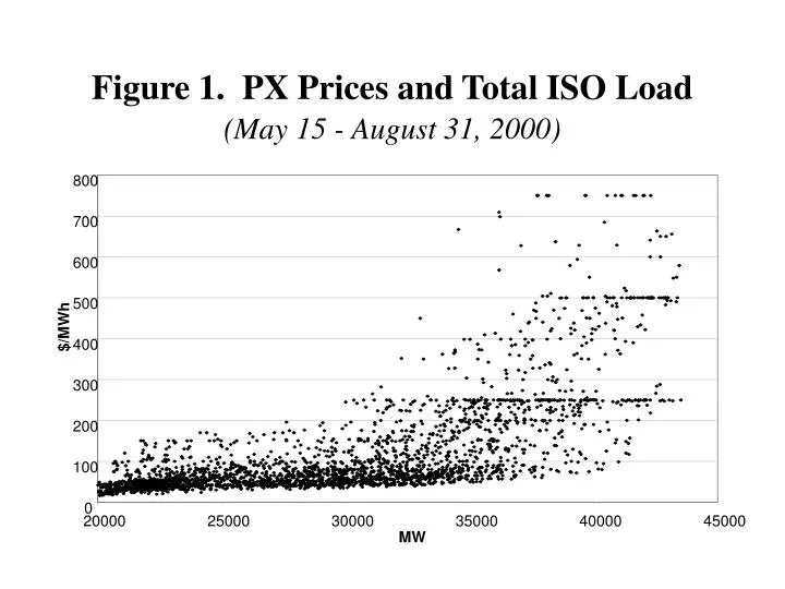
800. 700. 600. 500. $/MWh. 400. 300. 200. 100. 0. 20000. 25000. 30000. 35000. 40000. 45000. MW. Figure 1. PX Prices and Total ISO Load (May 15 - August 31, 2000). Figure 2. The Market Connected Demand Response in Steep Portion of Supply Curve Yields Lower Wholesale Prices.

E N D
800 700 600 500 $/MWh 400 300 200 100 0 20000 25000 30000 35000 40000 45000 MW Figure 1. PX Prices and Total ISO Load(May 15 - August 31, 2000)
Figure 2. The Market ConnectedDemand Response in Steep Portion of Supply Curve Yields Lower Wholesale Prices $/MWh Lnormal Lhot Pspike C B > > > > > > > E´ > Phot > Retail Price D > Pnormal A E Dhot Dnormal GWh Qnormal Qhot Qspike
1.00 20 0.80 16 Logarithm of P (in $/MWh) Normalized load 0.60 12 Load on highest price day 0.40 8 Highest prices 4 0.20 0 0.00 1 2 3 4 5 6 7 8 9 10 11 12 13 14 15 16 17 18 19 20 21 22 23 24 Hour Figure 3. RTP Load Response -- Moderate and High Prices (30% to 60% load reductions for most flexible customers)
1200 0.30 1000 0.25 800 0.20 600 0.15 400 0.10 200 0.05 0.00 0 Figure 4. Characterizing Hourly Price Responsiveness -- Flexibility Parameters Effect of Within-Day Flexibility Parameter -- One High-Price Hour • Ability to shift load within and between days • E.g., % shift in load within a day in response to given % change in relative price • Source of information--EPRI StatsBank Reference load FP = .10 FP = .25 RTP Price kWh $/kWh 1 2 3 4 5 6 7 8 9 10 11 12 13 14 15 16 17 18 19 20 21 22 23 24 Hour
Market share and demand responsiveness scenarios Low Medium High Demand response (MW) 484 1,065 1,935 (Percent of total ISO load) 1.2% 2.5% 4.6% Price reduction ($/MWh) $ 80 $ 160 $ 256 (Percent) 11% 24% 42% Cost reduction ($million) $ 3.3 $ 6.7 $ 10.8 Table 1. Effect of Demand ResponseOne hour at $750/MWh
Low Medium High Average price reduction, summer peak ($/MWh) $ 12.1 $ 24.5 $ 40.2 (Percent) 5.7% 11.6% 19.1% Total cost reduction, high- price days ($million) $ 344 $ 701 $ 1,158 (Percent) 4.7% 9.5% 15.7% Table 2. Total Effect of Demand ResponseMay - August 2000 (Alternative Scenarios)
35% 30% 25% 20% Market share of hourly pricing 15% 10% 5% 0% 0 0.05 0.1 0.15 0.2 0.25 0.3 Average price elasticity 24% price drop 42% price drop Figure 4. Sensitivity AnalysisTradeoff between Market Share and Price Responsiveness to achieve given price reduction (from $750/MWh)