Download
1 / 39
390 likes | 538 Vues
Recent Enhancements T owards C onsistent Credit Risk Modelling Across Risk Measures. RISK – Quant Congress USA 16-18 July 2014, New York. Péter Dobránszky.

E N D
Recent Enhancements Towards Consistent Credit Risk Modelling Across Risk Measures RISK – Quant Congress USA 16-18 July 2014, New York PéterDobránszky Disclaimer:The contents of this presentation are for discussion purposes only, representthe presenter’s views only and are not intended to represent the opinions of any firm orinstitution. None of the methods described herein is claimed to be in actual use.
Introduction • We investigate in this presentation the link between credit spread and rating migration evolutions • The first building block of a consistent modelling framework is the construction of appropriate generic credit spread curves • The main applications are VaR, IRC, CRM, CCR, CVA, etc. • Regulatory requirements for Regulatory CVA, credit VaR, wrong-way risk modelling, economic downturn modelling, incremental default in FRTB, etc. • We present a fully cross-sectional approach for building generic credit spread curves aka proxy spread curves • Difficulties with the intersection method – be granular but also robust and stable • Static representation vs. capturing the dynamics • Capturing times of stress and benign periods, stochastic business time, mean-reversions, regime switching modelling, etc. • Take into account risk premium, jump risk, gap risk, historical vs. risk neutral probabilities • Deal with observed autocorrelation
Assumptions We assume that we have a large enough history of spreads and corresponding ratings , where denotes a calendar date and identifies an issuer. We do not model the spread dynamics directly, but rather the log-spread dynamics. Accordingly, for convenience, we deal with in the following equations. These log-spreads If the data is not clean enough we may assign a weight for each issuer and for each day.
Least-square regression In the course of calibrating the rating distances we disregard the potential sector and region dimensions of the spreads and we will assume that the rating distances are static. Accordingly, we intend to calibrate the rating distances by the following regression.
Agenda • CDS curves • Capturing dynamics – sectorial approach (VaR, CVA VaR) • Factor analysis, Random Matrix Theory, Clustering • Estimating level – proxy spread curves (CVA, CS01, SEEPE) • Grouping • Rating migration effect (EEPE) • Migration matrix • Estimation error (IRC, CRM) • Default probabilities and recovery rate • Sovereigns (IRC, CRM) • Risk premium • Joint default events and correlated migration moves modelling • Concentration of events (IRC, CRM) • Some double counting issues
CDS curves • Understand the business cycles - stochastic business time (GARCH, etc.) • Detach business time (by sectors) from calendar time • VaR vs. Stressed VaR, EEPE vs. Stressed EEPE
CDS curves • Expected value of integrated business time over a calendar time period • Dynamics of ATM implied volatility for various maturities • Credit spreads as annual average default rates • Correlated, but standalone clocks
CDS curves • What is stationary? • Log-returns (?)
CDS curves • Capture the dynamics of spreads (VaR, CVA VaR, CRM) • Merge, demerge, new names • Illiquid curves – systemic, sectorial, idiosyncratic risk components • Selection of liquid curves as basis for capturing the dynamics • Definition of liquidity – contributors, number of non-updates • Sectorial approach – mappingof names to groups • Groups of names with similarities, homogeneity • Large enough and small enough groups, concentration • Trade-off between specificity and calibration uncertainty • Representation by number of names and by exposures • Can you assume cross-sectionalrelationships? • (N industry + M sector) systemic factors • (N industry ×M sector) systemic factors
CDS curves • Principal Component Analysis of CDS log-returns, decompose correlation • Biased figures if not accounted for stochastic business times • Assume a group of 10 with an extra 30% variance explanation within group • This specific group factor explains only of total variance
CDS curves • Assume 10 explanatory factors and remove their impact • Does the remaining part behaves like random independent noise? • Still there can be 50 groups of 10 names with an extra group factor explaining 30% of the variance within the group
CDS curves • Random Matrix Theory: it explains the eigenvalue distribution • If , with a fixed ratio , the eigenvalue spectral density of the correlation matrix is given by where . • But it works also for . For instance, .
CDS curves • Principal components are often misleading • If you have risk factors and you remove the impact of the first principal components, then the remaining variance is explained by only instead of factors. • Therefore, the first principal components explains also part of the noise variance. • Assume a one-factor model for 4 variables with pairwise correlations of 50% • Remove the impact of the first principal component – remaining parts of the 4 variables are not uncorrelated, instead, their correlation is -33%! – over-compensation • Remove the mean – mean captures only part of the systemic factor’s variance, thus the remaining parts of the 4 variables have a 6% correlation – under-compensation
CDS curves • Still mapping of clusters to sectors and regions are required • Not robust towards outliers, few small clusters and large concentration • Large clusters should be re-clustered • Does not ensure homogeneity within cluster – fixed number of clusters • Recent: Make 2 clusters, split each cluster into 2 until RMT conditions are met – still exposed to outliers • Clustering • It is a technique that collects together series of values into groups that exhibit similar behaviour. • Hierarchical clustering based on Euclidean distance or correlation
CDS curves • Estimating level for a given day – proxy spread curves (CVA, CS01, SEEPE) • Data mining like exploration • How many distinguishable groups are there? Split by how many dimensions? • Basel III requests split by sectors, regions and ratings (see EBA BTS)
CDS curves • Hypothesis test: difference between means • Apply the so-called two-sample t-test, which is appropriate when the following conditions are met: • The sampling method for each sample is simple random sampling. • The samples are independent. • Each sample is drawn from a normal or near-normal population. • The first two conditions are met by construction. Concerning the third rule, by rules-of-thumb, a sampling distribution is considered near-normal if any of the following conditions apply: • The sample data are symmetric, unimodal, without outliers, and the sample size is 15 or less. • The sample data are slightly skewed, unimodal, without outliers, and the sample size is 16 to 40. • The sample size is greater than 40, without outliers. • Analyse log-spreads and normalise by the rating effect
CDS curves • Two-sample t-test – compare groups based on two-tailed tests • Null hypothesis: considering two sectors, their average spread levels are equal. Alternative hypothesis: average spread levels are not equal, thus these sectors require separate proxy spread curves. • Assume that the standard deviations by samples are different. Therefore, compute the standard error (SE) of the sampling distribution as • The distribution of the statistic can be closely approximated by the t distribution with degrees of freedom (DF) calculated as • The test statisticis a t-score (t) defined by .
CDS curves P-values of the two-sample t-test as of 15 June 2012 P-values of the two-sample t-test as of 31 December 2008 • P-values • Grouping may change as sector levels fluctuate • Defines minimum number of names in a group • Here only European issuers, however, is it the same in NA? • Are there cross-sectional information being useful?
CDS curves • Useful cross-sectional information • Recently slope is not 1 As of 31 December 2008 As of 15 June 2012
CDS curves • Rating dependency for various sectors and regions • Different slope coefficients may be required • Bigger difference between sectors than regions
CDS curves Regulation, CRR, Article 158: (i) for institutions using the Internal Model Method set out in Section 6 of Chapter 6, to calculate the exposure values and having an internal model permission for specific risk associated with traded debt positions in accordance with Part Three, Title IV, Chapter 5, M shall be set to 1 in the formula laid out in Article 148(1), provided that an institution can demonstrate to the competent authorities that its internal model for Specific risk associated with traded debt positions applied in Article 373 contains effects of rating migrations; • Rating migration effect (EEPE) • BIS Quarterly Review, June 2004: “Rating announcements affect spreads on credit default swaps. The impact is more pronounced for negative reviews and downgrades than for outlook changes.”
Migration matrix • Estimation error (IRC, CRM) • Less or more rating matrices? Trade-off between capturing better the specific risk profiles and basic risk vs. reducing the estimation noise. • Which ones? Sovereign and corporate migration matrices? Corporate divided by region (US / Europe) and industry (financial / non-financial)? • Relevance for bank portfolio vs. availability of data, i.e. available data often with US concentration. • Finer rating grid may reduce the jump of P&Ls on the tails, but it introduces estimation noise. • Binomial proportion confidence interval, i.e. how reliable is the transition probability estimate? • CLT:, Wilson interval: • For a 95% confidence interval: • Enormous IRC impact • Smoothing?
Migration matrix • Calculation of short-term transition matrices • Markov approach: Assume time-homogeneous continuous-time Markov chain and scale the transition matrix via the generator matrix. • Which is the best short-term matrix which provides that multiplying it by itself several times gives the best approximation for the original one-year matrix? • = • Cohort method: Discrete-time method based on the historical migration data. Calibrations to various time horizons may show autocorrelation in migrations. • Maximum likelihood estimation assuming Markov model • Accounting for stochastic business times
Default probabilities and recovery rates • Source of recovery rates • What are the local currency recovery rates? • Sovereigns may go default on their hard currency and local currency obligations separately • Does the IRC engine simulate both events, if yes, how to manage correlation, if not, which rating is used for IRC calculations • It can be interpreted as what is the LC/HC bond value in case the HC/LC bond migrate or default • Various approaches to adjust the LC recovery rates to account for FX depreciation – quanto CDSs may be used • What are the recovery rates for covered bonds and government guarantees? • The rating of issuing bank is taken, which implies “high” PD, but when the issuer goes to default, there is still a pool of assets or another guarantor to meet the obligation. • Recovery rates are usually high to compensate that “wrong” PDs are used. • Ensure that bond PV < recovery rate
Default probabilities and recovery rates • Comparison of transformed historical PDs with Markit sector curves as of 30 June 2009 and assuming 40% recovery rate. • Taking non-diversifiable risk is compensated by premium. • The rarer the event the more difficult to diversify and the higher the risk premium. • IRC: historical PDs are used for simulations, while implied default probabilities are used for re-pricing. • Impact depends on the portfolio. • Source of estimated or implied probabilities of defaults (PD) • Historical TTC default probabilities provided by rating agencies (cohort). • Risk-neutral PIT default probabilities bootstrapped from traded CDSs.
Default probabilities and recovery rates • Accounting for risk premium • Banks take over risk, diversify and get compensation for systemic risk • Diffusion processes: risk premium over risk is negligible in the short-term • Risk premium related to jump risk and gap risk is priced differently • BB sector 5Y CDS ranged between 100 and 700 bps from beginning 2006 to mid 2011 • Implied default rate around 1.7-11% () vs. TTC default rate of 1% • Rare events (AAA) are priced with higher risk premium • Problems started to rise with Basel 2.5 • IRC loss distribution is strongly effected by risk premium • Visualise the potential time value effect when risk premium is significant
Default probabilities and recovery rates • Short protection portfolio of CDSs written on BB rated issuers • 30th June 2009 • Average 1Y CDS spread of the constituents was 600 bps • In case no default or migration event happens, expected portfolio P&L is around 6% • Not accounting for time value, expected portfolio P&L is around -1% (TTC) • Numerous default events may occur before any effective loss is realised
Joint default events and correlated migration moves j T T+∆t k Time fractions of co-movements • Asset value correlation: parameter of the Gaussian copula approach • Default correlation (Pearson correlation): • If CEDFj is not equal to CEDFk, the default correlation can never reach 100% • Process correlation: when processes are moving together
Asset value correlation model • Gaussian case • Pairwise correlations determine the whole joint dependence structure • Proxies for calibration • Factor correlation approach (KMV GCorr) • Same correlation for defaults and migrations • Copula: one-step discrete-time approach • Forward joint density does not exist
Term structure of default correlations • Fix the AVC and measure the Pearson default correlation for various horizons(annual PD = 2%, 2-state Markov chain with jump-to-default) • Similar term structure of default correlations by ratings • The lower the cumulative probability of defaults the lower is the default correlation • Most copula based approaches imply that the defaults of highly rated names are basically independent • Opposite to this, process correlations produce flat default correlation curves
Default correlations by rating classes different default correlation structure by rating term structure is flat at PC2 if T is small Gaussian copula AVC = 10% Correlated continuous-time Markov chains Process corr. = 11% Time fraction 1.2%
Event concentration – the new dimension of uncertainty j j k T+∆t T k T+∆t T l l High concentration Low concentration • In case of jumpy processes the parameterisation of the pairwise dependence structures is not enough to determine the N-joint law • Same pairwise dependence structure, but different N-joint law • High concentration: Armageddon scenario likely • Low concentration: probability of large number of defaults is high
Incremental modelling uncertainty Compare Gaussian copula model against more advanced correlated jump models with various event concentrations AVC = 8.5%, which means process correlation of 10% PD, LGD and P&L effect of rating changes are the same in each case Fixed time horizon of one year In case of small portfolios, various models produce very similar IRC loss distributions
Incremental modelling uncertainty The larger the portfolio the larger the impact of the model choice Especially short protection portfolios are very sensitive to the concentration modelling – concentration of default events can hardly be calibrated
Separating default and migration correlations • Until this point we assumed the same correlation between default events and migration moves. Nevertheless, we can separate the Markov generator matrix for defaults and migrations. • Even perfectly correlated migration moves cannot reproduce the realised default correlations • Critics for reduced-form models correlating only default intensities
Stochastic business time • Time homogeneity is clearly not an appropriate assumption • Stress periods are described by volatility clusters
Stochastic business time Recent time changed models are designed to explain default correlations Use a realistic statistical model to describe the business time dynamics
Stochastic business time • Calibrate the transition generator by assuming stochastic business time • What degree of realised default correlation can be explained by SBT? • Similarity with correlated default intensities (correlated migration only) • Default correlation by rating is not flat! Combine with process correlation! • Term structure of default correlation by PC = 11% plus SBT (hockey stick):
Some double counting issues • Consistency and coherency issues between capital charges • Potential exposure within a year does not capture that losses in case of a future default have potentially been realised already by CVA VaR when spreads were climbing up – this CVA variation is capitalised now • Similarly for IRC vs. VaR – if being long credit for Greece, daily MtM losses were capitalised by VaR, while there was no further loss at the time of default, thus IRC capital charge was questionable • Sudden and expected defaults shall be separated and capitalised accordingly