Strain II
Strain II. Mohr Circle for Strain. Recall that for stress, we plotted the normal stress n against the shear stress s , and we used equations which represented a circle


Strain II
E N D
Presentation Transcript
Mohr Circle for Strain • Recall that for stress, we plotted the normal stress n against the shear stress s, and we used equations which represented a circle • Because geologists deal with deformed rocks, when using the Mohr circle for strain, we would like to deal with measures that represent the deformed state (not the undeformed state!)
Equations for Mohr circle for strain • Let’s introduce two new parameters: ´ = 1/ (to represent the abscissa) ´ = / = ´ (to represent the ordinate) • The two equations for the Mohr circle are in terms of ´and ´ ´ = (´1+´3)/2–(´3-´1)/2 cos2´ ´ = (´3-´1)/2 sin2´
Mohr Circle for Strain • The coordinates of any point on the circle satisfy the above two equations • The Mohr circle always plots to the right of the origin because we plot the reciprocal quadratic elongation ’=1/ =(1+e)2, i.e., • =(1+e)2 and ´=1/ are both‘+’
Mohr Circle for Strain … • In parametric form, the equations of the Mohr circle are: ´ = c – r cos2´ ´ = r sin2´ Where: Center, c = (´1+´3)/2 (mean strain) Radius, r = (´3-´1)/2
Sign Conventions • The 2angle is from the c´1 line to the point on the circle • Points on the circle represent lines in the real world! • Since we use the reciprocal quadratic elongations´1 & ´3 • clockwise (cw) from c´1 is ‘+’, and • Counterclockwise ccw is ‘-’ (compare it with stress!) • cw in real world is cw 2 in the Mohr circle, and vice versa! • However, ccw, from the O´line to any point on the circle, is ‘+’, and cw is ‘-’
Lines of no finite elongation - lnfe • Draw the vertical line of lnfe =1 the ´axis • The intersection of this magic line with the Mohr circle defines the lnfe (there are two of them!). • Elongation along the lnfe is zero • They don’t change length during deformation, i.e., elnfe=0, and lnfe=1, and therefore ´lnfe=1 • Numerical Solution: tan2´ = (1-´1)/(´2-1)
Finding the angular shear • Because ´=/ and ´=1/ therefore: ´= ´which yields = ´/´ • Since shear strain, =tan, and = ´/´: tan =´/´ • Note: Mohr circle does not directly provide the shear strain or the angular shear , it only provides ´ • However, notice that ´= if ´=1!
Angular Shear = ´/´ • The above equation means that we can get the angular shear () for any line (i.e., any point on the circle) from the ´/´ of the coordinates of that point • Thus, is the angle between the ´ axis and a line connecting the origin to any point on the circle • ccw in the Mohr circle translates into ccw in the physical world (i.e., same sense)!
Finding the Shear Strain • The ordinate of the Mohr diagram is ´, not the shear strain • Because = ´/´, then = ´ only if ´=1 • This means that for a given deformed line (e.g., a point ‘A’ on the Mohr circle), the ´ coordinate of the intersection of the ‘magical’ ´=1 line with the OA line (connecting the origin to ‘A’) is actually because along the ´=1 line, and ´ are equal! • Procedure: • For any line (which is a point, e.g., ‘A’, on the circle), first connect the point ‘A’ to the origin (O), and extend the line OA (if needed), to intersect the ´=1 line • Read ´along the ´=1 line; this is for the line!
Finding lines of maximum shear (lms) strain (max) • Draw two tangents (±) to the Mohr circle from the origin, and measure the 2´(±) where the two lines intersect the circle • Numerical Solution: • Orientation: tan´lms=(2/1) (Note: these are,not´) • Amount: max =(1-2 )/2 12
ExampleA unit sphere is shortened by 50% and extended by 100% e1=1, and e3=-0.5 s1=X=l´/lo =1+e1=2 & s3=Z=l´/lo=1+e3=0.5 1 = (1+e1)2=s12 =4 &3=(1+e3)2 =s32=0.25 1´= 1/1=0.25 &3´= 1/3=4 • Note the area remains constant: XZ = 1 3= 40.25 =1 c =(´1+ ´3)/2 = (0.25+4)/2=2.125 r =(´3 - ´1)/2 = (4-0.25)/2=1.90 • Having ´c´ and ´r´, we can plot the circle!
Graphic representation of strain ellipse • Point A (1,1) represents an undeformed circle (1 = 2 = 1) • Because by definition, 1>2 , all strain ellipses fall below or on a line of unit slope drawn through the origin • All dilations fall on the 1 = 2 line through the origin • All other strain ellipses fall into one of three fields: • Above the 2=1 line where both principal extensions are + • To the left of the 1=1 where both principal extensions are – • Between two fields where one is (+) and the other (-)
Graphic representation of strain ellipse • Along AB, the original circle does not change shape but only change radius • From A to origin the radius gets smaller (l & 2<1) • Along AC: elongation along 1, and no change along 2 • Along AD: shortening along 2& no change along 1 • Only along the hyperbola through field 3, where 1= 1/2, is the area of the ellipse equal to the area of the undeformed circle (i.e., constant area) • Zone 3 is the only field in which there are two lnfes
Volume change on Flinn Diagram • Recall: S=1+e = l'/lo andev = v/vo =(v’-vo)/vo • An original cube of sides 1 (i.e., lo=1), gives vo=1 • Since stretch S=l'/lo, and lo=1, then S=l' • The deformed volume is therefore: v'=l'. l'. l' • Orienting the cube along the principal axes V' =S1.S2.S3 = (1+e1)(1+e2)(1+e3) Since v =(v’-vo), for vo=1 we get: v =(1+e1)(1+e2)(1+e3)-1
Given vo=1, since ev = v/vo, thenev = v =(1+e1)(1+e2)(1+e3) -1 • 1+ev =(1+e1)(1+e2)(1+e3) If volumetric strain, v = ev = 0, then: (1+e1)(1+e2)(1+e3) = 1 i.e., XYZ=1 • Express 1+ev =(1+e1)(1+e2)(1+e3) in e & take log: ln(1+ev) = e1+e2+e3 • Rearrange: (e1-e2)=(e2-e3)-3e2+ln(1+ev) • Plane strain (e2=0) leads to: (e1-e2)=(e2-e3)+ln(1+ev) [straight line: y=mx+b; with slope, m=1]
Ramsay Diagram • Small strains are near the origin • Equal increments of progressive strain (i.e., strain path) plot along straight lines • Unequal increments plot as curved plots • If v=evis thevolumetric strain, then: • 1+v =(1+e1)(1+e2)(1+e3) = lnS=ln(1+e) • It is easier to examine v on this plot Take log from both sides and substitute forln(1+e) • ln(v+1)=1+ 2+3 • If v>0, the lines intersect the ordinate • If v<0, the lines intersect the abscissa
Measurement of Strain • Originally circular objects • When markers are available that are assumed to have been perfectly circular and to have deformed homogeneously, the measurement of a single marker defines the strain ellipse
Direct Measurement of Stretches • Sometimes objects give us the opportunity to directly measure extension • Examples: • Boudinaged burrow • Boudinaged tourmaline • Boudinaged belemnites • Under these circumstances, we can fit an ellipse graphically through lines, or we can analytically find the strain tensor from three stretches
Direct Measurement of Shear Strain • Bilaterally symmetrical fossils are an example of a marker that readily gives shear strain • Since shear strain is zero along strain axes, inspection of enough distorted fossils (e.g. brachiopods, trilobites) can allow us to find the direction
Wellman's Method • Relies on a theorem in geometry that says that if two chords together cover 180° of a circle, the angle between them is 90° • In Wellmans method, we draw an arbitrary diameter of the strain ellipse • Then we take pairs of lines that were originally at 90° and draw them through the two ends of the diameter • The pairs of lines intersect on the edge of the strain ellipse
Fry’s Method • Depends on objects that originally were clustered with a relatively uniform inter-object distance. • After deformation the distribution is non-uniform • Extension increases the distance between objects; shortening reduces the distance • Maximum and minimum distances will be along S1 and S2, respectively
From: http://seismo.berkeley.edu/~burgmann/EPS116/labs/lab8_strain/lab8_2009.pdf
Fry’s Method; how to • Put a tracing paper on top of the objects, and mark their centers with a dot (this is the centers sheet) • On a second tracing paper, choose an arbitrary reference point (this is the reference sheet) • Place the reference point on top of the one dot (grain), and mark all other dots from the centers sheet onto the reference sheet • Place the reference point on a second dot, and copy all other dots • Repeat this for all dots
… • This lead to many dots, and the strain ellipse is defined either by: • an empty elliptical space around the reference point, or • an elliptical area full of points • Trace the approximation of the strain ellipse
Pros and cons • Fry’s Method is fast and easy, and can be used on rocks that have pressure solution along grain boundaries, with some original material lost • Rocks can be sandstone, oolitic limestone, and conglomerate • The method requires marking many points (>25) • The estimation of the strain ellipse’s eccentricity is subjective and inaccurate • If grains had an original preferred orientation, the method cannot be used
Rf/ Method • In many cases originally, roughly circular markers have variations in shape that are random • In this case the final shape Rfof any one marker is a function of the original shape Ro and the strain ratio Rs Rf,max = Rs.Ro Rf,min = Ro/Rs
http://a1-structural-geology-software.com/The_rf_phi__prog_page.htmlhttp://a1-structural-geology-software.com/The_rf_phi__prog_page.html
http://a1-structural-geology-software.com/The_rf_phi__prog_page.htmlhttp://a1-structural-geology-software.com/The_rf_phi__prog_page.html