Example: Control Flow Graphs
process Flowgraph = {. x : int, pc: {c 0 , c 1 , c 2 , c 3 , c 4 , c 5 } init pc = c 0 update pc = c 0 → x := 1 ; pc := c 1 pc = c 1 → pc := c 2 pc = c 2 ∩ x ≤ 100 → pc := c 3 pc = c 2 ∩ x > 100 → pc := c 5 pc = c 3 → x := x + 1 ; pc := c 4 pc = c 4 → pc := c 2. c 0.

Example: Control Flow Graphs
E N D
Presentation Transcript
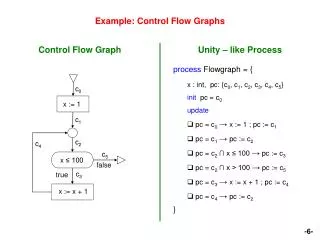
process Flowgraph = { • x : int, pc: {c0, c1, c2, c3, c4, c5} • init pc = c0 • update • pc = c0→ x := 1 ; pc := c1 • pc = c1→ pc := c2 • pc = c2∩ x ≤ 100 → pc := c3 • pc = c2 ∩ x > 100 → pc := c5 • pc = c3→ x := x + 1 ; pc := c4 • pc = c4→ pc := c2 c0 x := 1 c1 c2 c4 c5 x ≤ 100 false c3 true x := x + 1 } Example: Control Flow Graphs Control Flow Graph Unity – like Process -6-
Example: Mutual Exclusion P = m : cobegin P0 || P1coend m’ P0 :: l0 : while true do { nc0 : wait (turn = 0) cr0 : turn := 1 } l0’ : P = P0 || P1 P0 = { • turn : {0,1} , pc0 : { nc0, cr0} • init pc0 = nc0 • update • pc0 = nc0 ∩ turn = 0 → pc0 := cr0 • pc0 = nc0 ∩ turn = 1 → pc0 := nc0 • pc0 = cr0→ turn := 1 ; pc0 := nc0 } P1 :: l1 : while true do { nc1 : wait (turn = 1) cr1 : turn := 0 } l1’ : P1 = { • turn : {0,1} , pc1 : { nc1, cr1} • init pc1 = nc1 • update • pc1 = nc1 ∩ turn = 1 → pc1 := cr1 • pc1 = nc1 ∩ turn = 0 → pc1 := nc1 • pc1 = cr1→ turn := 0 ; pc1 := nc1 } Pseudo - code -7-
Example: Mutual Exclusion Expanded process P = { • turn : {0,1} , pc0 : { nc0, cr0} , pc1 : { nc1, cr1} • init pc0 = nc0∩ pc1 = nc1 • update • pc0 = nc0 ∩ turn = 0 → pc0 := cr0 • pc0 = nc0 ∩ turn = 1 → pc0 := nc0 • pc0 = cr0→ turn := 1 ; pc0 := nc0 • pc1 = nc1 ∩ turn = 1 → pc1 := cr1 • pc1 = nc1 ∩ turn = 0 → pc1 := nc1 • pc1 = cr1 → turn := 0 ; pc1 := nc1 } -8-
Q = int x arcs I = pc = c0 = { (x, c0) | x Є int } R = pc0 = c0 ∩ x’ = 1 ∩ pc’ := c1U pc = c1 ∩ pc’ := c2U pc = c2∩ x ≤ 100 ∩ pc’ := c3U pc = c2 ∩ x > 100 ∩ pc’ := c5U pc = c3 ∩ x’ = x + 1 ∩ pc’ := c4U pc = c4∩ pc’ := c2 ^ ^ Example: Transition Relation Unity – like Process Semantics type arcs = {c0, c1, c2, c3, c4, c5} process Flowgraph = { • x : int, pc: arcs • init pc = c0 • update • pc = c0→ x := 1 ; pc := c1 • pc = c1→ pc := c2 • pc = c2∩ x ≤ 100 → pc := c3 • pc = c2 ∩ x > 100 → pc := c5 • pc = c3→ x := x + 1 ; pc := c4 • pc = c4→ pc := c2 } -9-
post [ pc = 2 ∩ x ≤ 100 → pc := c3 ](φ) = pc’, x’ . pc’ = 2 ∩ x’ ≤ 100 ∩ pc = c3 ∩ φ(pc’, x’) pre [ pc = 2 ∩ x ≤ 100 → pc := c3 ](φ) = pc’, x’ . pc = 2 ∩ x ≤ 100 ∩ pc’ = 3 ═>φ(pc’, x’) = pc = 2 ∩ x ≤ 100 => φ[3/ pc’, x/ x’] E ~ A Example: Predicate Transformers -10-
SA = (QA,vTiA, I A) is an abstraction of S iff (1) Iγ(IA) (2) i, q Є QA . Post [ Ti ](γ(q)) γ(TiA(q)) A ΤiA γ γ Τi Abstract Semantics of Programs Abstract State Graphs: S = (Q,vTi, I) state graph of the program QAa lattice of abstract states α : P(Q) → QAα(γ(q)) = q γ : QA→ P(Q) φ ═>γ(α(φ)) A Galois connection given γ→ α(φ) = ∏ {q Є QA | φ => γ(q)} Consequence: every concrete execution is represented by at least one abstract -11-
Galois connection: γ(expA(B1, .., Bl)) = expA[φ/ B ] α(φ)= Λ {expA(B1, .., Bl )| φ═> expA[φ/ B ] } -not easily computed═> use apper approx (monomial) α’(φ)= Λ {(Bi | φ═> φi } l i = 1 Abstract State Lattice Main idea: Given {φ1, .. , φl} predicates on vars of concrete P. B1, .., Bl boolean variables (all concrete states that satisfy φi) Abstract states: set of predicates overB1, .., Bl(QA). Monomial on B1, .. , Bl: conjunction of Bi’s and ¬Bi’s (at most once) Theorem: The set M of monomials on B1 .. Bl forms: - complete lattice and (α ; γ) Galois connection -12-
false if expA[φ/ B ] ═> ¬qi(3.0) Bj if post[Ti ](expA[φ/ B ]) ═> φj(3.1) Λ ¬Bj ifpost[Ti ](expA[φ/ B ]) ═> ¬φj(3.2) true otherwise(3.3) l i = 1 Ti A (expA) = otherwise Abstract Transitions Main idea:Ti A (expA) = α(post[Ti ](γ(expA))) Ti A Problem: difficult to compute. α( post[Ti ]( γ(expA))) expA γ α Ti Ti A (expA) = α’(post[Ti ](γ(expA))) post[Ti ](γ(expA)) γ(expA) Use monomial approximation α’ of α. Has following form: By using (2.1) and (2.2) : (3.1)BjifexpA[φ/ B ] Λ qj ═> φj [ assi(x)/ x ] -13-
Abstract Successors Computing abstract successors: check validity of implications (3) - use a decision procedure (DP) - automatic theorem prover implementing such DPs. → for all i Є [1, .. , l ]. prove ( 3.0 | 3.1 | 3.2 ) Imposibility of proving (3): - post[Ti ](expA[φ/ B ]) intersects bothφj and ¬φj - abstract expA too big → cut in smaller pieces - because of monomials - abstract state space is too rough. - applied proof strategy is not powerful enough Abstract initial state: IA = α’(init) - in most practical cases, defines one value for most variables. - can be computed by evaluating φi -14-