Cost Behavior & Cost-Volume-Profit Analysis
210 likes | 871 Vues
Cost Behavior & Cost-Volume-Profit Analysis. David B. Hamm, MBA, CPA Managerial Accounting—Chs. 7 & 8 Fall, 2002. Cost Structures (Basic):. Fixed costs— do not vary with production levels in relevant range Variable costs— vary directly with sales and/or production activity

Cost Behavior & Cost-Volume-Profit Analysis
E N D
Presentation Transcript
Cost Behavior & Cost-Volume-Profit Analysis David B. Hamm, MBA, CPA Managerial Accounting—Chs. 7 & 8 Fall, 2002
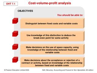
Cost Structures (Basic): • Fixed costs—do not vary with production levels in relevant range • Variable costs—vary directly with sales and/or production activity • Mixed costs—often typical, will contain elements of fixed and variable costs (example—utility costs usually contain a base service cost + a cost per kwh or cu.ft.) • Note—the key here is time and quantity—over the “long run,” all costs become variable, thus we look at a ‘relevant range’ of activity. But in the relevant range, we assume a linear relationship between cost and quantity (impacting VC and FC).
Contribution-format income statement (separate VC from FC) Note: all costs (production & general) are grouped by VC + FC in the contribution format.
How do you break down “Mixed” costs into Variable + Fixed costs? • Graphically—a “visual fit” line plotting points on a graph can estimate the slope of the line (slope= VC per unit) and the intercept—where the line crosses the base axis denotes FC. • Linear regression—challenging by hand but easy with spreadsheet functions, provides most reliable data. • Hi-Lo Method: Quick calculation may approximate regression results if data is consistent.
Motor, Inc. Data: Motor, Inc. compares maintenance cost with direct labor hours for the months of September-December (labor hours is deemed to be the driver for maintenance cost):
Scattergram with Trendline & Equation(Linear regression)—Excel Chart Wizard
What if we don’t have a computer handy? • The Hi-Lo method will do a quick calculation of the “end points” on the line to estimate slope & intercept: $14,000/8,000 = $1.75 per hour (slope or VC per hour)
Hi-Lo method (conclusion): Warning: The Hi-Lo method is an estimate only, using the high and low data points on a chart. If the high or low points are “irregular,” this method may not give an accurate estimation of the line (VC and FC may be off).
Break Even Analysis (1): • Because we can assume a correlation (linear relationship) between total costs and output— • FC is constant (in the relevant range) • VC is constant “per unit” (again in relevant range) • We can also assume total revenue is constant, or a constant price x quantity sold and thus also linear • Therefore, we can “chart” the break-even point, or the point where sales=total costs • See graph following
Break Even Analysis (3): • Why a “break even” point? Don’t we want to make a profit? • Yes, but establishing the b/e point enables us to determine the level of production and sales necessary to cover our total costs • Any sales level below b/e point is a loss • Any sales level above b/e point generates profit • Problem with graphics—a visual display, must have a computer or good graphics skills. Probably more accurate to do using basic algebra.
Break Even Analysis (4): The basic equation to find break even point is B/E Sales = Variable Costs + Fixed Costs Illustration: if selling price for widgets is $12 each, VC = $8 each and FC= $40,000 per month then b/e sales is: B/E = VC + FC 12 w = 8 w + 40,000 4 w = 40,000 w = 10,000 widgets
Break Even Analysis (5): We can alter the formula for any missing variable. For example, with previous data, suppose we fix production at 10,000 units per month, but don’t know what price to charge: B/E = VC + FC 10,000 p = 10,000 (8) + 40,000 10,000 p = 120,000 p = $12 (selling price per unit)
Break Even Analysis (6): Of course no firm wants to just break even. But we can easily change the model to insert a target profit, say $20,000 per month: B/E sales = VC + FC + Profit 12 w = 8 w + 40,000 + 20,000 4 w = 60,000 w = 15,000 widgets
Break Even Analysis (7): We can define a target profit as a profit per unit. Example- we want $2 profit per widget sold: B/E sales = VC + FC + Profit 12 w = 8 w + 40,000 + 2 w 2 w = 40,000 w = 20,000 widgets to be sold
Break Even Analysis (end) Finally, some accountants prefer to use the contribution approach, a “short cut” to the b/e formula: B/E point in units = Fixed Costs Unit contribution margin w = 40,000 / (12-8) (selling price – VC) w = 40,000 / 4 w = 10,000 widgets DBH suggestion—the S = VC + FC formula easily allows for substitutions or variations as discussed.
Forecasting Profit: If you know total FC and a VC per unit you can estimate profit using a contribution format income statement ( S = VC + FC + Profit) In a forecast, we can change any variables we wish to view alternative results
Sales Mix (1): What about multiple products (a sales mix)? If a consistent relationship can be found between two or more products, we can compute a weighted average contribution margin and break even point per product can be estimated. See next slide for illustration:
Cost Volume Profit Assumptions • Linear revenue behavior • No change in price over relevant range • Linear cost behavior • FC , VC per unit constant over relevant range • All costs are identifiable as fixed, variable, or mixed costs (can be estimated as FC + VC) • All production is sold—inventories are excluded from calculation End of Presentation