Chapter 12 The Chi-Square Test
Chapter 12 The Chi-Square Test. Used when there are two or more categories with qualitative data. Used to test for a relationship between categories We tested for relationship with quantitative data in Chapter 10. Chapter 12: Contingency Tables.

Chapter 12 The Chi-Square Test
E N D
Presentation Transcript
Chapter 12The Chi-Square Test • Used when there are two or more categories with qualitative data. • Used to test for a relationship between categories • We tested for relationship with quantitative data in Chapter 10.
Chapter 12: Contingency Tables • A quick way to look at this is that each participant is asked at least two questions that have qualitative answers. • At least one of the questions may have more than two possible answers.
Chapter 12: Contingency Tables Contingency Tables, or Cross Tabulation Tables, categorize two qualitative variables based on observed counts (frequencies) in each of several categories. Examples: Course Letter Grade and Gender, Political Affiliation and Support/Non-support for a candidate State of birth and Political Affiliation College Major and Plans for highest degree (Bachelor’s, Master’s, or Ph.D.)
Chapter 12: Contingency Tables • The main question is: are the answers to the questions related (dependent) are they not related (independent) • We test for this by seeing if the percentage of answers is the same for all groups. • (The number of answers will be different depending on the size of the samples, that is why we test the percentages.)
Chapter 12: Test for Independence The question is whether the two variables are independent. Test H0: Variables are independent. vs Ha: Variables are dependent. Example: Consider Favorite Subject vs. Gender. What is meant by independence? Basically, is the percentage the same for each group? An example of independence might be: Favorite Subject Area Row GenderMath/ScienceSocial ScienceHumanitiesTotals Male 40(40%) 40(40%) 20(20%) 100 Female 80(40%) 80(40%)40(20%) 200 Column Totals 120 120 60 300 Male/Math/Sci = 40 out of 100 = 40% Female/Social Science = 80 out of 200 = 40% Now let’s look at an example that’s not so simple and figure out how we would answer the question in general.
Chapter 12: Test for Independence Test H0: Variables are independent. vs Ha: Variables are dependent. Calculate % based on row totals. (ie: 122 males and 178 females) Favorite Subject Area Row GenderMath/ScienceSocial ScienceHumanitiesTotals Male 37(30%) 41(34%) 44(36%) 122 Female 35(20%) 72(40%)71 (40%)178 Column Totals 72 113 115 300 Male/Math/Sci = 37 out of 122 = 30%
Chapter 12: Test for IndependenceIf Gender and Favorite Subject are independent, then the expected cell frequency is just the row total multiplied by the column total divided by the number in the sample. • Favorite Subject Area Row • GenderMath/ScienceSocial ScienceHumanitiesTotals • Male 37 41 44 122 • Female 35 72 71 178 • Column Totals 72 113 115 300 We expect how many in the Male-Social Science category? 122 x 113 = 13,786. Then 13,786 divided by 300 is 45.95. We expect how many in the Female-Humanities area? 178 x 115 = 20470. Then 20470 divided by 300 is 68.23.
Chapter 12: Contingency Tables • If two qualitative variables are truly independent of each other, then the observed cell counts should be “close to” the expected cell counts. • If they are not independent, the difference between them will be relatively large. • So we need to measure the difference. • Then, to make these measurements comparable throughout the table, we will divide by the expected to see what the percent of difference is. • Once we have done this for all the cells, we add these numbers to get the test statistic, which we call chi-square.
Chapter 12: Contingency Tables We can compare the observed cell frequencies to what we expected to see. If this value is small, there is little reason to doubt the null hypothesis. If this value is large, this suggests the variables are related, or dependent, and there is support for the alternative hypothesis. c2 = is our test statistic. It has a chi-square distribution with df=(r-1)(c-1) where r= # of rows and c = # of columns for each application when all the Expected Cell Frequencies are at least 5.
Chi-Square Distribution • This is a new distribution. • We have previously worked with z, t, and F distributions. • Chi-Square distribution looks different, but does use degrees of freedom. • The Χ2 table (Table 7) page 591 gives us the p value if we know Chi-Square and the number of degrees of freedom.
Chapter 12: Test for Independence Typically, the expected cell frequencies are listed in parentheses within the table. (We will utilize Minitab to find the expected cell frequencies.) Favorite Subject Area Row GenderMath/ScienceSocial ScienceHumanitiesTotals Male 37(29.28) 41(45.95) 44(46.77) 122 Female 35(42.72) 72(67.05)71(68.23)178 Column Totals 72 113 115 300 The test statistic can then be computed. = 4.604 To get the p-value, we would use a chi-square table (Table 6)(df = 2) The test statistic and the p-value will be obtained from StatCrunch.
Chapter 12: Test for Independence We will use StatCrunch to perform the calculations. Enter the columns of your table into StatCrunch (You must keep track of the rows). Use STAT Tables Contingency Enter the columns containing the table and click OK The next slide has the table, with expected counts and “contributions to the chi-square” test statistic. We will focus on: expected cell counts – are they all 5 or more? (validity) chi-square – report the value as the test statistic’s value. p-value – If this is less than a, we will accept Ha.
Note: All expected cell frequencies are greater than 5, so the method is valid. We would fail to accept the alternative hypothesis, and thus conclude there is insufficient evidence at the .05 level of significance that the two variables are dependent.
Chapter 12: Contingency Tables • If we conclude that two qualitative variables are dependent, we must be careful not to say that one causes the other. We are just saying that they are statistically dependent. (show up in those groupings in the population). • We could not say that having math as a favorite subject causes one to be male.
12.2 Describing the relationship • If the hypothesis testing shows that there is a relationship between one variable and another (dependent), the next step is to describe the relationship. Of course, it there is no relationship, this step is not needed.
12.2 Describing the relationship • If the experimenter wished to compare the categories of Variable A, the percentage of responses for every category of Variable B should be calculated for each category of Variable B.
12.2 Describing the relationship • Favorite Subject Area Row • GenderMath/ScienceSocial ScienceHumanitiesTotals • Male 37(30%) 41(34%) 44(36%) 122 • Female 35(20%)72(40%)71 (40%)178 • Column Totals 72 113 115 300 • Male/Math/Sci = 37 out of 122 = 30% • If we were to just look at these percentages: • Favorite Subject Area Row • GenderMath/ScienceSocial ScienceHumanitiesTotals • Male 30% 34% 36% 100% • Female 20%40%40%100% • We can say that more favorite subject area is just about evenly divided for males, but females favor Social Science and the Humanities over Math/Science.
12.2 Describing the relationship • When interpreting the percentages, to experimenter must remember that they describe the relationship in the sampled observations. • Whether or not we can then draw conclusions about the populations they represent depends upon how well the samples were selected.
12.2 Describing the relationship • Remember, the higher the p-value, the more independent the relationship. • Low p-values allow us to accept the alternative hypothesis that the two variables are dependent. • So the differences are not due to chance, but show a real relationship between the variables.