
Normal Distribution
E N D
Presentation Transcript
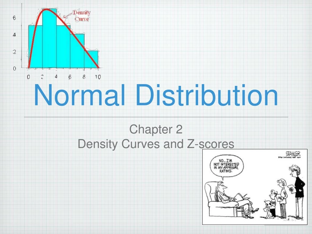
Normal Distribution • Chapter 2 • Density Curves and Z-scores
CASE STUDY: The new SAT In March 2005, the College Board administered the new SAT for the first time. Students, parents, teachers, high school counselors, and college admissions officers waited anxiously to hear about the results from this new exam. Would the scores on the new SAT be comparable to those from previous years? How would students perform on the new Writing section (and particularly on the timed essay)? In the past, boys had earned higher average scores than girls on both the Verbal and Math sections of the SAT. Would similar gender differences emerge on the new SAT? By the end of this chapter, you will have developed the statistical tools you need to answer important questions about the new SAT.
Case Study 2.1 Suppose that Thabang earns an 86 (out of 100) on his next statistics test. Should he be satisfied or disappointed with his performance?
Here are the scores of all 25 students in Mr. E’s stat class: The bold score is Thabang’s: 86. How did he perform on this test relative to his classmates?
Stemplot Where does Thabang’s 86 fall relative to the center of this distribution? Since the mean and median are both 80, we can say that Thabang’s result is “above average.” But how much above average is it?
If x is an observation from a distribution that has known mean and standard deviation, the standardized value of x is A standardized value is often called a z-score. Measuring Relative Standing: z-Scores One way to describe Thabang’s position within the distribution of test scores is to tell how many standard deviations above or below the mean his score is.
= 80 X s = 6.07 N ( 80, 6.07 )
Naomi Jeremy T-BANG Thabang’s score on the test was x = 86. His standardized test score is: Naomi’s score on the test was x = 93. Her standardized test score is Jeremy’s score on the test was x = 72. His standardized test score is
Thabang: 0.99 X Naomi: 2.14 Jeremy: -1.32 Their scores under the density curve Jeremy: -1.32 Thabang: 0.99 Naomi: 2.14
Standard Notation N(µ,∂) µ = mean ∂ = standard deviation
Practice SAT versus ACT Eleanor scores 680 on the mathematics part of the SAT. The distribution of SAT scores in a reference population is symmetric and single-peaked with mean 500 and standard deviation 100. Gerald takes the American College Testing (ACT) mathematics test and scores 27. ACT scores also follow a symmetric, single-peaked distribution but with mean 18 and standard deviation 6. Find the standardized scores for both students. Assuming that both tests measure the same kind of ability, who has the higher score? Show your work and draw the density curve distribution.
Answer Eleanor: z = (680 − 500)/100 = 1.8 Gerald: z = (27 − 18)/6 = 1.5 Eleanor′ s score is higher.