Download
1 / 20
200 likes | 533 Vues
The NCAR TIE-GCM: Model Description, Development, and Validation. Alan Burns, Barbara Emery, Ben Foster, Gang Lu, Astrid Maute, Liying Qian, Art Richmond, Ray Roble, Stan Solomon, and Wenbin Wang High Altitude Observatory National Center for Atmospheric Research.

E N D
The NCAR TIE-GCM:Model Description, Development, and Validation Alan Burns, Barbara Emery, Ben Foster, Gang Lu, Astrid Maute, Liying Qian, Art Richmond, Ray Roble, Stan Solomon, and Wenbin Wang High Altitude Observatory National Center for Atmospheric Research Chapman Conference • Charlestown, South Carolina • 10 May 2011
Thermosphere-Ionosphere-ElectrodynamicsGeneral Circulation Model (TIE-GCM) • Original development by Ray Roble, Bob Dickinson, Art Richmond, et al. • The atmosphere/ionosphere element of CMIT and the CISM model chain • Cross-platform community release (v. 1.93), under open-source academic research license • v. 1.94 release, May 2011 • User manual complete • Documentation mostly complete • Runs-on-request at CCMC
Development History • Thermosphere General Circulation Model • TGCM, 97~500 km, Dickinson et al., 1981; 1984; Roble et al., 1982 • Thermosphere-Ionosphere General Circulation Model • TIGCM, 97~500 km, Roble et al.,1987; 1988 • Thermosphere-Ionosphere-Electrodynamics General Circulation Model • TIE-GCM , 97~500 km, Richmond et al., 1992;Richmond, 1995 • Thermosphere-Ionosphere-Mesosphere-Electrodynamics GCM • TIME-GCM, 30~500 km, Roble and Ridley, 1994; Roble, 1995 • Whole Atmosphere Community Climate Model • WACCM, 0~140 km, Marsh et al., 2007; Garcia et al., 2007 • Extended Whole Atmosphere Community Climate Model • WACCM-X, 0~500 km, Liu et al., 2010
Equations • Momentum equation: u, v • Continuity equation: w, O, O2, N(4S), NO, O+ • Hydrostatic equation: z • Thermodynamic equation: TN, Te • Quasi-steady state energy transfer—electron, neutral, ion: TI • Photochemical equilibrium: N(2D), O2+,N2+,N+,NO+ Coordinate system: horizontal: rotating spherical geographical coordinates; vertical: pressure surface (hydrostatic equilibrium) Resolution:horizontal: 5°x 5°; vertical: 0.5 pressure scale height. High resolution version (2.5° x 2.5° x H/4) in test.
Numerical Techniques • Horizontal: explicit 4th order centered finite difference; • Time: 2nd order centered difference; • Vertical: Implicit 2nd order centered difference; • Shapiro filter: achieve better numerical stability; • Fourier filter: remove high frequency zonal waves generated by finite difference (high latitudes)
External Forcing of the Thermosphere/Ionosphere System • Solar XUV, EUV, FUV (0.05-175 nm) • Default: F10.7-based solar proxy model (EUVAC). • Optional: solar spectral measurements, other empirical models. • Solar energy and photoelectron parameterization scheme (Solomon & Qian, 2005) • Magnetospheric forcing • High latitude electric potential: empirical models (Heelis et al., 1982; Weimer, 2005), or data assimilation models (e.g., AMIE), or magnetosphere model (CMIT) • Auroral particle precipitation, analytical auroral model linked to potential pattern (Roble & Ridley, 1987) • Lower boundary wave forcing • Tides: Global Scale Wave Model (GSWM , Hagan et al, 1999) • Eddy diffusion
Boundary Conditions • Upper boundary conditions: • u, v, w, TN, O2, O: diffusive equilibrium; • N(4S),NO: photochemical equilibrium; • O+:specify upward or downward O+flux; • Te: specify upward or downward heat flux. • Lower boundary conditions: • u, v: specified by tides (GSWM) • TN: 181 K + perturbations by tides (GSWM) • O2: fixed mixing ratio of 0.22 • O: vertical gradient of the mixing ratio is zero • N(4S), O+: photochemical equilibrium • NO: constant density of (8x10⁶) • Te: equal to TN.
ITM coupling: Electrodynamics • Low and mid-latitude: neutral wind dynamo equations solved on geomagnetic apex coordinates. [Richmond et al., 1992; 1995] • High latitude: specified by convection models such as Heelis, Weimer, and AMIE, or coupled to the LFM Magnetosphere Model.
Some Model Validation Examples • Thermosphere • Neutral density data from satellite drag • Neutral density data from CHAMP • Composition data from GUVI • Ionosphere • Electron density measurements from COSMIC • Ground-based incoherent scatter radar measurements • Ground-based GPS data
Thermospheric Density—Declining Phase of SC #23 [Qian et al., J. Geophys. Res., 2009]
Thermosphere Neutral Density, 2007 Ascending Descending CHAMP MSIS00 TIE-GCM
Electron Density Profiles 03/30/2007 06/21/2007 ISR ISR Model TIE-GCM LT=12 LT=15
Current Development and Future Plans • • TIE-GCM v. 1.94 is undergoing benchmark tests and will be released soon • • Significant new feature is inclusion of the Weimer high-latitude potential model, using solar wind / IMF input • • High-resolution version (2.5° x 2.5° x H/4) is also in test • • Other key research developments include: • • Lower boundary conditions: • — Seasonal/spatial variation of lower boundary eddy diffusion • — Tidal forcing derived from TIMED TIDI & SABER data • • External forcing: • — Solar EUV from TIMED/SEE, SDO/EVE, and alternative proxies • — Auroral precipitation derived from GUVI data • • Global Ionosphere Plasmasphere (GIP) model (closed field lines) • • Continued development of the Coupled Magnetosphere-Ionosphere-Thermosphere (CMIT) model • • More information at: http://www.hao.ucar.edu/modeling/tgcm
Strengths and Weaknesses Strengths: • Fully coupled neutral dynamics and ionospheric electrodynamics • Accurate treatment of solar EUV and photoelectron processes, including capability of using EUV measurements • Comprehensive photochemistry and thermodynamics • Flexible high latitude inputs: Heelis, Weimer, AMIE, or coupling to magnetospheric models (CISM/CMIT) Weaknesses: • Lower boundary — only migrating tides included • Upper boundary — no plasmasphere • Uniform spherical grid — problems near the poles • Hydrostatic equilibrium assumed
Infrared Cooling • CO2 cooling at 15 µm (peaks ~ 120 km) • NO cooling at 5.3 µm (peaks ~ 150 km)) • O(3P) fine structure cooling at 63 µm (maximizes > 200 km)
Thermosphere (O/N2) TIE-GCM GUVI 04/01 06/21