Oligopoly: Competition Among the Few
410 likes | 660 Vues
Oligopoly: Competition Among the Few. Assumptions for a “Hypothetical”. The Cournot Oligopoly Model. The Bertrand Oligopoly Model. Other Oligopoly Models. Return. Hypothetical Facts and Monopoly Result. 1000. 900. 800. 700. 600. P = 950 - Q. Monopoly Price = 500. 500. 400. MR. 300.

Oligopoly: Competition Among the Few
E N D
Presentation Transcript
Oligopoly: Competition Among the Few Assumptions for a “Hypothetical” The Cournot Oligopoly Model The Bertrand Oligopoly Model Other Oligopoly Models Return
Hypothetical Facts and Monopoly Result 1000 900 800 700 600 P = 950 - Q Monopoly Price = 500 500 400 MR 300 200 MC = 50 100 0 0 100 200 300 400 500 600 700 800 900
Monopolist’s Profit-maximizing Output Q P MR Rev Tcost Profit 445 505 60 224,725 22,250 202,475 446 504 58 224,784 22,300 202,484 447 503 56 224,841 22,350 202,491 448 502 54 224,896 22,400 202,496 449 501 52 224,949 22,450 202,499 450 500 50 225,000 22,500 202,500 451 499 48 225,049 22,550 202,499 452 498 46 225,096 22,600 202,496 453 497 44 225,141 22,650 202,491 454 496 42 225,184 22,700 202,484 455 495 40 225,225 22,750 202,475 456 494 38 225,264 22,800 202,464 457 493 36 225,301 22,850 202,451 458 492 34 225,336 22,900 202,436 459 491 32 225,369 22,950 202,419 460 490 30 225,400 23,000 202,400
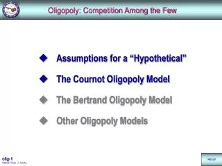
The Cournot Oligopoly Model Who (or What) Is “Cournot”? Premises of the Cournot Model Mathematical Cournot Model A Topographical Cournot Model Deriving the Reaction Curves The “Solution” of the Model Efficiency Properties: The Well Revisited
Hypothetical Facts and Monopoly Result 1000 900 800 700 600 P = 950 - Q Monopoly Price = 500 500 400 MR 300 200 MC = 50 100 0 0 100 200 300 400 500 600 700 800 900 Return
Antoine Augustin Cournot (1801-1877) Recherches sur les Principes Mathématiques de la Théorie des Richesses (1838) Regardez le Croix d’Honneur
Premises of Cournot Oligopoly Model • A few firms produce goods that are either perfect substitutes (homogeneous) or imperfect substitutes (differentiated). • Firms set output, as opposed to price. The market sets price where demand equals the amount supplied. • Each firm believes its rivals will hold output constant if it changes its own output.
Mathematical Approach • p = a-bQ • c(q) = cq , constant marginal cost • Firm i’s profit : (a-b(q-i +qi))qi - cqi • FOC: a-bq-i -2bqi - c = 0 • qi = (a-bq-i - c)/2b = R(q-i), i’s reaction • Cournot Equilibrium: qi = R(q-i) for all i. • n equations in n unknowns. • But all firms are alike, use symmetry: qi=q • Reaction: q = (a-b(n-1)q - c)/2b • q = (a -c)/b(n+1) • Q = (a-c)/b n/(n+1) • (a-c)/b as n . Competitive outcome!
Profits of Firm #1 – 3D View, Filled Bird’s Eye View
Profits of Firm #1 – Birds-eye View, Filled 900 800 700 600 500 190 Q1 400 170 300 150 130 200 110 90 70 100 50 30 10 0 0 100 200 300 400 500 600 700 800 900 Q2 Unfilled Topographic
Profits of Firm #1 – Birds-eye View, Unfilled 900 800 700 600 500 190 Q1 400 170 300 150 130 200 110 90 70 100 50 30 10 0 0 100 200 300 400 500 600 700 800 900 Q2 Firm #2
Profits of Firm #2 – 3D View 3D Firm #1 Bird’s Eye View
Profits of Firm #2 – Birds-eye View 900 800 700 600 500 Q1 400 300 200 100 50 10 110 90 70 30 130 170 150 190 0 0 100 200 300 400 500 600 700 800 900 Q2 Unfilled Topographic
Profits of Firm #2 – Birds-eye View, Unfilled 900 800 700 600 500 Q1 400 300 200 100 50 10 110 90 70 30 130 170 150 190 0 0 100 200 300 400 500 600 700 800 900 Q2
Reaction Curves • Economists often use “Reaction Curves.” Where did we see this before? • In the Cournot case, the reaction curve for one firm plots its output decisions against various outputs for the other firm(s).
Profits of Firm #2 – Birds-eye View, Unfilled 900 800 700 600 500 Q1 400 300 200 100 50 10 110 90 70 30 130 170 150 190 0 0 100 200 300 400 500 600 700 800 900 Q2
Deriving Firm #2’s Reaction Curve 900 800 700 600 500 Q1 400 300 200 100 50 10 110 90 70 30 130 170 150 190 0 0 100 200 300 400 500 600 700 800 900 Q2
Deriving Firm #1’s Reaction Curve 900 800 700 600 500 190 Q1 400 170 300 150 130 200 110 90 70 100 50 30 10 0 0 100 200 300 400 500 600 700 800 900 Q2
Summary: Reaction Functions • Firm 1’s reaction (or best-response) function indicates the amount of Q1 that firm 1 should produce in order to maximize its profits for each possible quantity of Q2 produced by firm 2. • Since the products of the two firms are substitutes, an increase in firm 2’s output leads to a decrease in the profit-maximizing amount of firm 1’s product.
Intersection of Reaction Curves 190 170 150 130 110 90 70 50 30 10 900 800 700 600 Q1 500 400 300 200 100 90 110 130 50 30 10 170 70 150 190 0 0 100 200 300 400 500 600 700 800 900 Q2
Adjustments Toward Equilibrium When Firm Two Enters 900 800 700 Firm #2’s Best-Reaction Curve 600 Q1 500 400 Redo 300 200 Firm #1’s Best-Reaction Curve 100 0 0 100 200 300 400 500 600 700 800 900 Q2
Stable Equilibrium, Expectations Confirmed 900 800 700 600 Q1 500 400 300 200 100 0 0 100 200 300 400 500 600 700 800 900 Summary Q2
Cournot Equilibrium • Situation where each firm produces the output that maximizes its profits, given the the output of rival firms • No firm can gain by unilaterally changing its own output
Questions • Is the Cournot Equilibrium also a Nash Equilibrium? • Is the Cournot Equilibrium an efficient result for the firms? Nash Equilibrium
Nash Equilibrium The intersection of the reaction curves corresponds to a Nash equilibrium because • this result involves output combinations at which the profits of each firm are maximized, given its expectations about output from the other firm(s); • and the outputs expected by all firms are indeed being produced by the other firm(s). That is, the expectations are validated by experience.
But . . . A Nash Equilibrium is not always an “efficient” result for the players.
Area to be “Zoomed” 900 800 700 Q1 600 500 400 170 300 130 200 90 100 50 40 100 70 10 160 130 190 10 0 0 100 200 300 400 500 600 700 800 900 Q2
Zoomed Version 500 10 10 400 40 170 300 70 100 200 130 130 90 100 160 10 50 40 190 10 0 0 100 200 300 400 500 Q1 Simplified Q2
Simplified Diagram Showing Cournot Equilibrium 500 400 Q1 300 78.8 90.0 101.2 200 112.4 112.4 101.2 90.0 78.8 100 0 0 100 200 300 400 500 Analogue Q2
Similar to the “Well Problem” 500 400 Q1 300 78.8 90.0 101.2 200 112.4 112.4 101.2 90.0 78.8 100 0 0 100 200 300 400 500 Well Problem Q2
Cournot vs. Collusive Result Q1+Q2=450 500 400 Q1 300 90.0 101.2 200 112.4 112.4 101.2 90.0 78.8 100 0 0 100 200 300 400 500 Equilibrium? Q2
Collusive Result Unstable? Q1+Q2=450 500 400 Q1 300 90.0 101.2 200 112.4 112.4 101.2 90.0 78.8 100 0 0 100 200 300 400 500 Monopoly Result Q2
Nash Equilibrium A Nash equilibrium is a set of strategies, one for each player, such that no player has an incentive to unilaterally change her action. Players are in equilibrium if a change in strategies by any one of them would lead that player to earn less than if she remained with her current strategy. Return