Download
1 / 11
110 likes | 209 Vues
This study aims to create a fine-scale hourly rainfall product by combining radar and special rain gauge measurements. It includes details on the CHARM rain gauge network, NWS WSR-88D products, case study intercomparison, data combination, and more. The analysis compares data from the CHARM network with WSR-88D radar data, providing insights on rainfall patterns and accuracy. Findings suggest potential for improving precipitation estimates through data integration.

E N D
Intercomparison of CHARM Data and WSR-88D Storm Integrated Rainfall Gary Jedlovec (NASA), Paul Meyer (NASA), Anthony Guillory (NASA), Ashutosh Limaye (USRA), Global Hydrology and Climate Center,Huntsville, Alabama and Keith Stellman (NOAA/NWS), LMRFC, Slidell, Louisiana • Goal: Produce a fine scale hourly rainfall product by combining radar and special rain gauge measurements. • Outline: • CHARM rain gauge network • NWS WSR-88D HDP products • Case study intercomparison • Data combination • Discussion
COOPERATIVE HUNTSVILLE-AREA RAINFALL MEASUREMENT NETWORK (CHARM) GAUGE OWNERSHIP MAP 80km JANUARY 2002 • Local precipitation network ( est. 1/2001) • 110 sites in Huntsville & Madison County, AL • NASA, Army, USGS, and NWS sites and weather enthusiasts • Daily rainfall totals (1200UTC reports) • 3600 km2 coverage (1 gauge per 6x6 km) • Primarily 4” manual gauges (70%) with remaining (30%) manual or automated tipping bucket (6” and 8”) • Plans to expand to 200 stations by 2003 • 4x4 km average spacing • twice daily manual observations • 1 minute data from 40 automated sites http://wwwghcc.msfc.nasa.gov/charm big picture • Supports local weather and climate research at the GHCC • validate weather radar and lightning data from satellites • monitor spatial distributions of precipitation for modeling activities • various satellite remote sensing studies of soil moisture and energy fluxes
TYPES OF RAIN GAUGES USED IN CHARM 4” non-recording “all-weather” plastic 6”, 8” non- recording (metal) 6”, 8” tipping bucket – recorded electronically 6”, 8” recording weekly paper charts
CHARM Data Analysis • June 4-5, 2001 Case Study • Isolated heavy thunderstorm moves • through the CHARM network • Slow west-to-east movement over Huntsville Rainfall totals reported at 1200UTC for the preceding 24h . For June 4-5, the 24h totals capture only this storm event. Irregularly spaced gauge data (from 200m to 10 km) were objectively analyzed to a uniform grid to create the image. Some smoothing of maximum values is inevitable. Max= 2.96” Max=2.73” Maximum rain rate of about 2 in/hr • Details: • Strong north-south gradient on • either side of the storm track. • Width of heavy rainfall area is • about 10 km • Maximum of 2.96” on east of • region, secondary max (2.73”) in • the western half of network big picture
NASHVILLE RADAR HYTOP RADAR Hourly Digital Precipitation Product • NWS offices produce their own precipitation estimatesfrom their local WSR-88D radar. The Nashville and Hytop (northeast of Huntsville) radars captured this storm event. • Figures present storm totals (sum of hourly product over storm lifetime ~ 4-6 hours). • Same general structure • Nashville radar depicts more intense and • widespread rainfall • Radar calibration, elevation, scan patterns and • distance from storm may all contribute to the • difference. 4-5” ~3”
NWS HDP Products Example of stage III radar product for June 4, 2001 over Northern Alabama. Hourly stage III product summed from 2100 – 0300 UTC. • Stage I - integrated precipitation from local radar using standard or tropical Z-R relationships on • 4 km grid – dependent on Z-R relationship used • Stage II - adjusted stage I product for bias using local (hourly) rain gauges • Stage III - combination of stage II HDP from individual radars to produce a regional precipitation estimate • minimal bias due to mis-calibration and different Z-R, local and seasonal adjustments • regional continuity and consistency Rainfall (cm) Note the dual rainfall maximum in the stage III radar product corresponds nicely both in position and magnitude to the CHARM data. Stellman et al. 2001 (Wea. Fore.) CHARM
Stage III versus CHARM • Resolution issues will affect comparison • Radar: • radar volume – varies with distance • 4km grid cells – arbitrary selection • Rain gauge: • point measurement – microscale variability of rainfall greatest in convective situations • multiple rain gauges for each grid cell (a single best comparison used in analysis below) ALL POINTS MD = 0.19” SD = 0.50” Comparison shows little or no bias (0.19”) between CHARM measurements and radar estimates. Scatter is considerable especially for amounts > 1.00”. <1” > 1” MD = 0.21” 0.17” SD = 0.15” 0.60”
Combined Stage III and CHARM Data Can time-continuous stage III data products be used to improve on 24h precipitation estimates from spatially dense CHARM rain gauge network? • Adjust hourly stage III data using CHARM 24h data • Assume rain gauge (24h total) is correct and assume (radar – rain gauge) bias is constant with time • Calculate bias between stage III data and CHARM 24h amount on a gauge-to-radar (4km data cell) basis • Use point-to-point bias to scale (or “adjust”) stage III data Actual gauge values • For NSSTC site, bias factor was 1.36 (radar under-estimate). • Rainfall duration is spread over wider span • Adjustment produces radar under-estimate
Combined Radar – Rain Gauge Product - Summary • Individual radar estimates of precipitation vary greatly from radar-to-radar without some bias adjustment. • The NWS stage III HDP product which uses (a few) regional rain gauges to adjust radar estimates of precipitation for calibration and Z-R inaccuracies shows considerable improvement in precipitation estimation. • Hourly radar rainfall estimates can be used to increase the utility of daily precipitation measurements (24h totals) from gauges by applying local bias corrections and radar time estimates. However, as a result • the duration of the rain event is often over estimated by up to 2dt • (2 hours for this study), • 2) the duration over estimate will lead to an storm intensity underestimate • Despite these minor shortcomings, the combined radar and gauge rainfall product has a variety of uses for meso/microscale studies.
GAUGE OWNERSHIP MAP 80km back JANUARY 2002