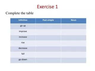
Exercise 1
Exercise 1. You have a clinical study in which 10 patients will either get the standard treatment or a new treatment Randomize which 5 of the 10 get the new treatment so that all possible combinations can result. Use Excel or R or another formal randomization method.

Exercise 1
E N D
Presentation Transcript
Exercise 1 • You have a clinical study in which 10 patients will either get the standard treatment or a new treatment • Randomize which 5 of the 10 get the new treatment so that all possible combinations can result. Use Excel or R or another formal randomization method. • Instead, randomize so that in each pair of patients entered by date, one has the standard and one the new treatment (blocked randomization). • What are the advantages of each method? • Why is randomization important? SPH 247 Statistical Analysis of Laboratory Data
Exercise 1 Solutions • For the first situation, using Excel, you can (for example) put the numbers 1–10 in column A, put five “Treatment” and five “Standard” in column B, put =rand() in column C. Then fix the numbers in column C and sort columns B and C by the random numbers. • For the second situation, you can put random numbers in column B and fix them, then in cell C2 (assuming a header row) put =IF(B2<B3,"A","B") and in cell C3 put =IF(B3<B2,"A","B"). Then copy the pair of cells to C4, C6, C8, and C10. Or use “Treatment” and “Standard” instead of “A” and “B”. • There are many other ways to do this. SPH 247 Statistical Analysis of Laboratory Data
Before Sorting After Sorting SPH 247 Statistical Analysis of Laboratory Data
Comments • Randomization is important to avoid bias, approximately balance covariates, and provide a basis for analysis. • Blocked randomization can better control for time effects, but this particular version risks unblinding the next patient. SPH 247 Statistical Analysis of Laboratory Data
Exercise 2 • Analyze the testosterone levels from Rosner’sendocrin data set in the same way as we did for the estradiol levels, using anova(lm()) • Reanalyze estradiol and testosterone using lme() and verify that the results are the same. Here is the specificationlme(Testosterone ~ 1, random = ~1 | Subject,data=endocrin) • Repeat the analysis of the coop data for specimens 2 and 5 separately. Do the analysis both with the traditional ANOVA tables using lm() and with lme() and compare the results SPH 247 Statistical Analysis of Laboratory Data
> anova(lm(Testosterone ~ Subject,data=endocrin)) Analysis of Variance Table Response: Testosterone Df Sum Sq Mean Sq F value Pr(>F) Subject 4 571.66 142.915 22.041 0.002246 ** Residuals 5 32.42 6.484 --- Signif. codes: 0 ‘***’ 0.001 ‘**’ 0.01 ‘*’ 0.05 ‘.’ 0.1 ‘ ’ 1 Replication error variance is 6.484, so the standard deviation of replicates is 2.55 pg/mL This compared to average levels across subjects from 15.55 to 36.25 Estimated variance across subjects is (142.915 − 6.484)/2 = 68.2155 Standard deviation across subjects is 8.26 pg/mL If we average the replicates, we get five values, the standard deviation of which is 8.45. This contains both the subject and replication variance. SPH 247 Statistical Analysis of Laboratory Data
> lme(Estradiol ~ 1, random = ~1 | Subject,data=endocrin) Linear mixed-effects model fit by REML Data: endocrin Log-restricted-likelihood: -28.41785 Fixed: Estradiol ~ 1 (Intercept) 14.99 Random effects: Formula: ~1 | Subject (Intercept) Residual StdDev: 8.434606 2.458254 Number of Observations: 10 Number of Groups: 5 > lme(Testosterone ~ 1, random = ~1 | Subject,data=endocrin) Linear mixed-effects model fit by REML Data: endocrin Log-restricted-likelihood: -28.51958 Fixed: Testosterone ~ 1 (Intercept) 25.3 Random effects: Formula: ~1 | Subject (Intercept) Residual StdDev: 8.259258 2.546372 Number of Observations: 10 Number of Groups: 5 SPH 247 Statistical Analysis of Laboratory Data
Specimen 2 > anova(lm(Conc ~ Lab + Lab:Bat,data=coop,sub=Spc=="S2")) Analysis of Variance Table Response: Conc Df Sum Sq Mean Sq F value Pr(>F) Lab 5 4.6640 0.93280 150.52 4.947e-14 *** Lab:Bat 12 1.3951 0.11626 18.76 9.484e-08 *** Residuals 18 0.1115 0.00620 The test for batch-in-lab is correct, but the test for lab is not—the denominator should be The Lab:Bat MS, so F(5,12) = 0.93280/0.11626 = 8.0234 so p = 0.00157, still significant The residual variance is 0.00620 (sd=0.0787). The estimated batch variance within labs is (0.11626 −0.00620)/2 = 0.05503 (sd = 0.2346). The estimated lab variance is (0.93280 − 0.11626)/(3×2) = 0.13609 (sd = 0.3689) SPH 247 Statistical Analysis of Laboratory Data
> lme(Conc ~1, random = ~1 | Lab/Bat,sub=Spc=="S2",data=coop) Linear mixed-effects model fit by REML Data: coop Subset: Spc == "S2" Log-restricted-likelihood: 7.383694 Fixed: Conc ~ 1 (Intercept) 0.3658333 Random effects: Formula: ~1 | Lab (Intercept) StdDev: 0.3689019 Formula: ~1 | Bat %in% Lab (Intercept) Residual StdDev: 0.2345892 0.07872243 Number of Observations: 36 Number of Groups: Lab Bat %in% Lab 6 18 The standard deviations for Lab, Batch, and Residual exactly match those from the lm() analysis SPH 247 Statistical Analysis of Laboratory Data
Specimen 5 > anova(lm(Conc ~ Lab + Lab:Bat,data=coop,sub=Spc=="S5")) Analysis of Variance Table Response: Conc Df Sum Sq Mean Sq F value Pr(>F) Lab 5 16.3277 3.2655 33.7688 1.539e-08 *** Lab:Bat 12 7.2049 0.6004 6.2088 0.0003072 *** Residuals 18 1.7406 0.0967 --- Signif. codes: 0 ‘***’ 0.001 ‘**’ 0.01 ‘*’ 0.05 ‘.’ 0.1 ‘ ’ 1 The test for batch-in-lab is correct, but the test for lab is not—the denominator should be The Lab:Bat MS, so F(5,12) = 3.2655/0.6004 = 5.4389 so p = 0.00766, still significant The residual variance is 0.0967 (sd=0.3110). The estimated batch variance within labs is (0.6004 −0.0967)/2 = 0.2519 (sd = 0.5018). The estimated lab variance is (3.2655 − 0.6004)/(3×2) = 0.4442 (sd = 0.6665) SPH 247 Statistical Analysis of Laboratory Data
> lme(Conc ~1, random = ~1 | Lab/Bat,sub=Spc=="S5",data=coop) Linear mixed-effects model fit by REML Data: coop Subset: Spc == "S5" Log-restricted-likelihood: -30.32728 Fixed: Conc ~ 1 (Intercept) 7.761389 Random effects: Formula: ~1 | Lab (Intercept) StdDev: 0.6664803 Formula: ~1 | Bat %in% Lab (Intercept) Residual StdDev: 0.5018488 0.3109703 Number of Observations: 36 Number of Groups: Lab Bat %in% Lab 6 18 The standard deviations for Lab, Batch, and Residual exactly match those from the lm() analysis SPH 247 Statistical Analysis of Laboratory Data