Random variables
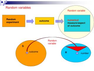
Random variables. Random variables and probability distributions Discrete random variables (Continuous random variables). Random variables. The term random variable refers to a numerical outcome of a random phenomenon .

Random variables
E N D
Presentation Transcript
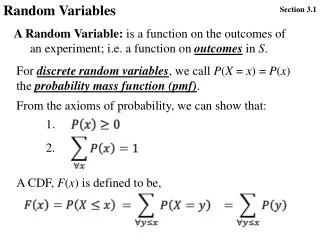
Random variables • Random variables and probability distributions • Discrete random variables • (Continuous random variables)
Random variables The term random variablerefers to a numerical outcome of a random phenomenon. • Example A: Toss a coin 3 times and let X be the number of heads. • X is a random variable whose possible values are 0, 1, 2, and 3. • Example B: Let Y be a number chosen using R’s runif(n) function. • Y is a random variable whose possible values are the numbers between 0 and 1. • Example C: Take a SRS of size 25 from the population of UNC undergrads and let W be the average GPA of the sampled students. • W is a random variable whose possible values are the numbers in the interval from 0.00 to 4.00.
Random variables • Any random variable has a set of possible values. Subsets of that set are events, and probabilitiesare assigned to the events. • Just like a probability model, except that the sample space must be a set of numbers. • This assignment of probabilities is the probability distributionof the random variable. • There are two kinds of random variable: • A discreterandom variable has a finite set of possible values. • A continuousrandom variable has a set of possible values that is an interval of real numbers.
Random variables • To specify the probability distribution of a discreterandom variable, we list the possible values along with the probability assigned to each. • Just like a finite sample space, except that with a random variable, the outcomes are always numbers. • To specify the probability distribution of a continuousrandom variable, we give a density curve over the interval of possible values. • Then the probability of any event is the area under the density curve, over the points in the event.
Discrete random variables Example 1a(based on Ex. 4.12, p. 238): Choose a number at random from a table of data that follows Benford’s Law. Let X = first digit. Then X is a discrete random variable. Its possible values X are 1,2,3,4,5,6,7,8,9, and the probability distribution is: A probability histogram of the distribution:
Discrete random variables Example 1b : Choose a digit at random. If 0, discard and draw again. Let Y be the digit chosen. Then the possible values of Y are 1,2,3,4,5,6,7,8,9, and the probability distribution is: A probability histogram of the distribution:
Discrete random variables Examples 1a and 1b: What is the probability that a digit is 3 or less… a. if the digit comes from data following Benford’s Law? b. if the digit comes from a table of random digits (with 0 discarded)? Benford: Random digits, 0 excluded:
Discrete random variables Toss a fair coin 4 times, and let X be the number of heads. The possible values of X are 0,1,2,3, and 4. To find their probabilities, we look at the sample space for the random phenomenon (i.e., 4 tosses of a coin), and we find the probabilities of the events “X=0”, “X=1”, etc. Sample space has 16 outcomes: HHHH HHHT HHTH HHTT HTHH HTHT HTTH HTTT THHH THHT THTH THTT TTHH TTHT TTTH TTTT Probabilities assigned to these: 1/16 each. We are interested in the probabilities of the five events “X = 0,” “X = 1,” etc. What are these events? “X = 1,” for example, is the event {HTTT, THTT, TTHT, TTTH}. Continued →
Discrete random variables Example 4.23, continued: The 16 outcomes: HHHH HHHT HHTH HHTT HTHH HTHT HTTH HTTT THHH THHT THTH THTT TTHH TTHT TTTH TTTT Arranged by the value of X (X = number of H’s): X = 0: TTTT X = 1: HTTT THTT TTHT TTTH X = 2: HHTT HTHT HTTH THHT THTH TTHH X = 3: HHHT HHTH HTHH THHH X = 4: HHHH So the probability distribution of X is:
Discrete random variables Example: X = number of rooms in a randomly-chosen house occupied by owner (San Jose, CA, 1998). Probability distribution of X: • Express the event “unit has 6 or more rooms” in terms of X and give its probability. • Express the event “X > 6” In words and give its probability. • c. What important fact about discrete random variables is illustrated by these two probabilities?
Continuous random variables • A continuous random variablehas all the numbers in an intervalas its possible values. Events are subsets of that interval. • The distributionof a continuous random variable is given by a density curve– a curve above the interval of possible values with a total area of 1. The probability of any event is the area under the density curve and above values in the event.
Continuous random variables One distribution that a continuous random variable might have: Standard Normal. Suppose Z has this distribution. Then probabilities of events involving Z are areas under the standard Normal density curve. Example: The probability that Z is between 1.4 and 2.2 is ______ – ______ = 0.0669 , because that is the area under the standard Normal curve above the interval from 1.4 to 2.2.
Continuous random variables Another distribution that a continuous random variable might have: uniform between 0 and 1. If X has this distribution, then probabilities of events involving X are areas under the horizontal ‘curve’ shown. Example: The probability that X is between 0.3 and 0.9 is 0.6, because that is the area under the uniform density curve above the interval from 0.3 to 0.9.
Continuous random variables Exercise 4.63, p. 259: Suppose we have a random variable Y whose distribution is uniform between 0 and 2. The density curve is then a horizontal straight line between 0 and 2. a. What is the height of the density curve? Draw a graph. b. What is P(Y ≤ 1.5)? c. What is P(0.6 < Y < 1.7)? d. What is P(Y ≥ 0.9)?
Distributions Relation between data distributions (Section 1.3) and probabilitydistributions (Section 4.3): Suppose the distribution of values in a population has a certain density curve. (That is, its histogram is well approximated by that curve.) If X is a random value taken from the population, then the probability distribution of X has that same density curve. So probabilities for X (i.e., for one “random draw” from the population)are the same as proportions in the population. For example, P(X < 50) is just the proportion of values under 50 in the population.
Discrete vs. continuous random variables A discrete random variableX can take on any value in a finite set of possible values, and each value in the set has a positive probability. A continuous random variable X can take on any value in an interval of possible values, but the probability of any single value in the interval is zero!. Example 1: If X is the number of heads in 4 tosses of a fair coin, then X is discrete. Its possible values are 0,1,2,3,4. P(X = 2) = 6/16, and therefore P(X ≥ 2) and P(X > 2) are different. (They differ by 6/16). Example 2: If X is the height of a randomly-chosen adult male, then X is continuous. Its possible values fill an interval (from the smallest possible height to the largest). P(X = 72”) = 0 (no one is exactly72.000000000000… inches tall), and therefore P(X ≥ 72) and P(X > 72) are equal.
The meanof a random variable Example: Suppose the distribution of X is If we repeat the random phenomenon many times and record all the values of X that we observe, what can we expect the average of our observations to be? Will it be the average of the possible values of X? That is (0+1+2)/3 = 1. Would our observations have an average of 1? NO! The average of many observations of X can be expected to be close to (0)(0.5) + (1)(0.3) + (2)(0.2) = 0 + 0.3 + 0.4 = 0.7. Why? →
The meanof a random variable If the distribution is why would we expect the average of many observations to be (0)(0.5) + (1)(0.3) + (2)(0.2)? Because a large number of observations of X will include about 50% zeroes, 30% ones, and 20% twos. Imagine making 10,000 observations of X and recording the results. The list of observed values would include about ________ zeroes, ________ ones, and ________ twos. The average of those 10,000 observed values would be about _______________________________. Meanof a random variable represents its expected long-run average value.
The meanof a discreterandom variable If X is a discrete random variable, the mean(or expected value) of X is denoted μX and defined as μX =x1p1+ x2p2+ x3p3+ ∙∙∙+ xkpk where x1, x2, …, xkare the possible values of X and p1, p2, …, pkare their probabilities. The sum above is sometimes written as Σxi pi .
The meanof a discreterandom variable Example 1: If you bet a dollar in a certain version of the game Chuck-a-luck, and X is your net gain or loss from that bet, then the distribution of X is So your expected gain or loss is μX= ____________. If you play many times, you can expect to lose an average of about ______ per play. If you play 1000 times, you can expect to lose about __________.
Example • You entered the following bet – gain $9 if an event happen (A=“UNC wins NCAA title”), loose $1 if the event A does not happen. • What is the expected winning/loss? • What probability P(A)=p leads to positive expected winning? (p>0.1)
Simplified roulette • Roullette has numbers (00),0,1,…36. • If you bet x on a number you get 35x if win on –x if loss. • Complications due to minimum and maximum bet are ignored. • What is the expected loss?
Dubins & Savage Problem • You are given initial wealth $100 • You can place any bets on the simplified roullette (European) • Play until either bust or reach $200 • What strategy would you use?

