Predation model predictions
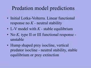
Predation model predictions. Initial Lotka-Volterra. Linear functional response no K - neutral stability L-V model with K - stable equilibrium No K, type II or III functional response - unstable

Predation model predictions
E N D
Presentation Transcript
Predation model predictions • Initial Lotka-Volterra. Linear functional response no K - neutral stability • L-V model with K - stable equilibrium • No K, type II or III functional response - unstable • Hump shaped prey isocline, vertical predator isocline - neutral stability, stable equilibrium or prey extinction
Paradox of enrichment (Rosenweig 1971 Science 171:385-387) …depends on the assumption of a vertical predator isocline
Modified - hump prey isocline: Instead of a hump, the prey isocline may be expected to rise at low prey populations because: - prey may find spatial refuges from predation at low densities (type III functional response) - prey may immigrate into habitat containing low prey numbers - kinked hump isoclines are inherently stable - predators can consume prey only down as far as the remaining prey population present in refuges or to the levels maintained by immigration (where prey isocline approaches vertical)
Changing the predator numerical response: • Have so far assumed the predator numerical responseV • (per capita growth rate of predators as function of prey abundance) is a linear function of prey abundance • - Seems reasonable to assume that predators also have carrying • capacities determined by factors other than prey availability. • - In state space, a carrying capacity will bend the predator zero • growth isocline to the right (more prey does not increase • predator numbers) • - This will generate a stable equilibrium along the horizontal • part of the predator isocline
Predator carrying capacity: predator can no longer drive prey to extinction. Stable coexistence
What happens if a predator has multiple prey? - Outcome will depend on whether prey species cycle in concert - If prey abundances are not strongly positively correlated then as one prey species becomes scarce, the predator can continue to feed and increase its population size. Unstable equilibrium predators drive prey to extinction
Predator carrying capacity and multiple prey species: Predator isocline with a positive slope is stable (damped oscillations) Any factor that rotates the prey or predator isocline in a clockwise direction will tend to stabilize interactions
Additional modifications to predator - prey models So far assumed that responses of predators to prey (and vice versa) are instantaneous. More realistic that predator population sizes will lag somewhat behind prey populations (the time required for consumed prey to be transformed into new predators) Incorporating time lags into models generally has a destabilizing effect leading to larger oscillations in predator/prey populations.
Conclusions: predation models • Simple predation models can generate a variety of behaviors - Neutral stability, stable limit cycles, and equilibrium stability. • Adding predator or prey carrying capacities tends to stabilize models whereas incorporating non-linear functional responses and time lags generally leads to instability. • Multiple prey species can destabilize populations if it allows predators to over-exploit prey, but predation may also facilitate prey coexistence (Paine paper) - depending on predator preference and competitive interactions among prey species • Simple lab predator-prey experiments most often result in extinction over a short time. This perhaps indicates the importance of refuges from predators in natural systems
Cyclic dynamics of the arctic collared lemming Gilg et al. (2003) Lemming populations show superannual cycles suggestive of predator prey dynamics
Measured lemming densities, over several years, and predation rates (observations, skat samples, pellet samples, lemming fur in borrows) Skua Fox Functional response Lemmings eaten/day Lemming density
Skua Fox Numeric response Young produced/yr Stoat Stoats occupy lemming nests in winter. Only predator to show a delayed response - highest number year after lemming pop peak Numeric response
Observed data Model prediction
Conclusions: No space or food limitation for lemmings ie no prey density-dependence (resource limitation) Only predation regulates lemming populations Dynamics generated by destabilizing predation by the stoat (time lag effects) and stabilizing effects by other predators (density dependent effects) Delayed numerical response of stoat driving force for numerical fluctuations Can use the model to examine effects of removing one or more predators on prey population dynamics
What about examples when food does become limiting? - Most famous example is cycling of Canadian lynx and snoe-shoe hare (Elton and Nicholson 1942, Journal of Animal Ecol 11:215) - Hare populations cycle with peak abundance ~ every 10 yr - Major source of hare mortality is predation - Lynx populations appear to closely track hare populations often peaking 1-2 years after the hare peak
Classic example of Lotka-Volterra neutral stability? Various hypotheses: Elton - variation in solar radiation resulting from periodic sunspot activity Keith (1963) Wildlife’s ten year cycle. Univ Wisconsin Press: Starvation/disease at high population sizes or predation?
Lemming-style predator-prey model does not work: - On Anticosti Island, Quebec there are no lynx but hare populations cycle anyway… Keith (1983,1984) Oikos 40:385-395; Wildlife Monog. 90:1-43 looked at the cycle in detail and concluded: Hare populations are co-limited by food availability and by predation from many sources (goshawks, owls, weasels, foxes, Coyotes). Hare population growth rates are sufficient to produce rapid depletion of food resources (principally buds and stems of shrubs and saplings). Furthermore, induced defenses of hare forage results in additional declines in food availability
Krebs et al. 1995 • Definitive study of snoeshow hare dynamics in Yukon • Only way to understand this system is through multifactorial manipulation experiment • 1 km2 plots. Monitoring of populations for 8 years • Fertilizer to increase plant growth (N,P,K) • Electric fences to keep large predators out (permeable to hares) • Food addition treatments • Predator exclusion - 2x hare density • Food addition - 3x hare density • Predator x Food addition - 11 x hare density • Some unresolved questions: mechanism? Why hares low so long?
Refuges from predation: Gause (1934) set out to look for evidence of population cycles between Paramecium and Didinium in a microcosm experiment. - Didinium quickly consumed all the Paramecium and then went extinct. -When sediment was placed in the bottom of the microcosm Paramecium was able to hide, Didinium went extinct and Paramecium population recovered. - Ability of prey to escape predators suggests that dispersal could within a metapopulation could provide opportunities for prey and predators to coexist
Huffaker (1958) Experimental studies on predation: dispersion factors and predator-prey oscillations Hilgardia 27:343-83 -Looked at populations of the six-spotted mite (Eotetranychus) that feeds on oranges and the predatory mite (Typhlodromus) -prey mite disperses by foot or by ballooning on silk strands -predator mites disperse on foot - Set up arrays of oranges with mini launch-pads on them for prey mite dispersal. - In large arrays predators and prey coexisted and showed population oscillations
Several examples of plants constrained to refuges by insect herbivores - coming soon to a discussion group!
Predation escape through predator satiation: If predation rates decline at high prey densities (type II and III functional responses) then predator satiation may allow prey species to maintain their populations. Many examples: Janzen suggested that seed predation is a major selective force favouring ‘masting’ (massive super-annual seed production) e.g. Janzen (1976) Why bamboos wait so long to flower. Ann. Rev. Ecol. Syst. 7:347-391 Bamboos are the most dramatic mast fruiters, with many species Fruiting at 30-50 yr intervals and some much longer e.g. Phyllostachysbambusoides fruits at 120 year intervals! Other masters: oaks, beech, conifers, Tachigali
Tachigali spp. “Suicide tree” Monocarpic - only dicot canopy tree in the world with this trait Large trees reproduce synchronously ~ every 5 years Seeds often lost to predispersal predation Trees infected by decay fungus before death (murder not suicide??)
Williams et al (1993) Predator satiation by periodical cicadas Ecology 74:1143-1152 Magicicada spp emerge once every 13 or 17 yrs up to 4 million/ha = 4 tonnes of cicadas/ha - the highest biomass of a natural population of terrestrial animals ever recorded! - Monitored Cicada populations in N. Arkansas - Estimated emergence rates by capturing insects in traps on the ground as they came out of the soil - Captured dead adults in traps and determined predation rate by birds by counting discarded wings
- Estimated 1,063,000 cicadas emerged in 16 ha - 50% of population emerged on just four nights - Birds killed a large proportion of the first emergents when Populations were low, but only killed 15 % of the population overall