Markov Random Fields
Markov Random Fields. Allows rich probabilistic models for images. But built in a local, modular way. Learn local relationships, get global effects out. MRF nodes as pixels. Winkler, 1995, p. 32. MRF nodes as patches. image patches. scene patches. image. F ( x i , y i ). Y ( x i , x j ).


Markov Random Fields
E N D
Presentation Transcript
Markov Random Fields • Allows rich probabilistic models for images. • But built in a local, modular way. Learn local relationships, get global effects out.
MRF nodes as pixels Winkler, 1995, p. 32
MRF nodes as patches image patches scene patches image F(xi, yi) Y(xi, xj) scene
Network joint probability 1 Õ Õ = Y F P ( x , y ) ( x , x ) ( x , y ) i j i i Z , i j i scene Scene-scene compatibility function Image-scene compatibility function image neighboring scene nodes local observations
In order to use MRFs: • Given observations y, and the parameters of the MRF, how infer the hidden variables, x? • How learn the parameters of the MRF?
Outline of MRF section • Inference in MRF’s. • Gibbs sampling, simulated annealing • Iterated condtional modes (ICM) • Variational methods • Belief propagation • Graph cuts • Vision applications of inference in MRF’s. • Learning MRF parameters. • Iterative proportional fitting (IPF)
Gibbs Sampling and Simulated Annealing • Gibbs sampling: • A way to generate random samples from a (potentially very complicated) probability distribution. • Simulated annealing: • A schedule for modifying the probability distribution so that, at “zero temperature”, you draw samples only from the MAP solution. Reference: Geman and Geman, IEEE PAMI 1984.
3. Sampling draw a ~ U(0,1); for k = 1 to n if break; ; Sampling from a 1-d function • Discretize the density function 2. Compute distribution function from density function
x2 x1 Gibbs Sampling Slide by Ce Liu
Gibbs sampling and simulated annealing Simulated annealing as you gradually lower the “temperature” of the probability distribution ultimately giving zero probability to all but the MAP estimate. What’s good about it: finds global MAP solution. What’s bad about it: takes forever. Gibbs sampling is in the inner loop…
Iterated conditional modes • For each node: • Condition on all the neighbors • Find the mode • Repeat. Described in: Winkler, 1995. Introduced by Besag in 1986.
Variational methods • Reference: Tommi Jaakkola’s tutorial on variational methods, http://www.ai.mit.edu/people/tommi/ • Example: mean field • For each node • Calculate the expected value of the node, conditioned on the mean values of the neighbors.
Outline of MRF section • Inference in MRF’s. • Gibbs sampling, simulated annealing • Iterated condtional modes (ICM) • Variational methods • Belief propagation • Graph cuts • Vision applications of inference in MRF’s. • Learning MRF parameters. • Iterative proportional fitting (IPF)
y1 x1 y2 x2 y3 x3 Derivation of belief propagation
y1 y3 y2 x1 x3 x2 The posterior factorizes
y1 y3 y2 x1 x3 x2 Propagation rules
y1 y3 y2 x1 x3 x2 Propagation rules
Belief, and message updates j = i j i
Optimal solution in a chain or tree:Belief Propagation • “Do the right thing” Bayesian algorithm. • For Gaussian random variables over time: Kalman filter. • For hidden Markov models: forward/backward algorithm (and MAP variant is Viterbi).
y1 y3 y2 x1 x3 x2 Y ( x , x ) 1 3 No factorization with loops!
Justification for running belief propagation in networks with loops Kschischang and Frey, 1998; McEliece et al., 1998 • Experimental results: • Error-correcting codes • Vision applications • Theoretical results: • For Gaussian processes, means are correct. • Large neighborhood local maximum for MAP. • Equivalent to Bethe approx. in statistical physics. • Tree-weighted reparameterization Freeman and Pasztor, 1999; Frey, 2000 Weiss and Freeman, 1999 Weiss and Freeman, 2000 Yedidia, Freeman, and Weiss, 2000 Wainwright, Willsky, Jaakkola, 2001
Statistical mechanics interpretation U - TS = Free energy U = avg. energy = T = temperature S = entropy =
Free energy formulation Defining then the probability distribution that minimizes the F.E. is precisely the true probability of the Markov network,
Approximating the Free Energy Exact: Mean Field Theory: Bethe Approximation : Kikuchi Approximations:
Bethe Approximation On tree-like lattices, exact formula:
Gibbs Free Energy Set derivative of Gibbs Free Energy w.r.t. bij, bi terms to zero:
Belief Propagation = Bethe Lagrange multipliers enforce the constraints Bethe stationary conditions = message update rules with
i Region marginal probabilities i j
Belief propagation equations Belief propagation equations come from the marginalization constraints. i i j = i j i
Results from Bethe free energy analysis • Fixed point of belief propagation equations iff. Bethe approximation stationary point. • Belief propagation always has a fixed point. • Connection with variational methods for inference: both minimize approximations to Free Energy, • variational: usually use primal variables. • belief propagation: fixed pt. equs. for dual variables. • Kikuchi approximations lead to more accurate belief propagation algorithms. • Other Bethe free energy minimization algorithms—Yuille, Welling, etc.
Update for messages Kikuchi message-update rules Groups of nodes send messages to other groups of nodes. Typical choice for Kikuchi cluster. i j i j = i j i = k l Update for messages
Generalized belief propagation Marginal probabilities for nodes in one row of a 10x10 spin glass
References on BP and GBP • J. Pearl, 1985 • classic • Y. Weiss, NIPS 1998 • Inspires application of BP to vision • W. Freeman et al learning low-level vision, IJCV 1999 • Applications in super-resolution, motion, shading/paint discrimination • H. Shum et al, ECCV 2002 • Application to stereo • M. Wainwright, T. Jaakkola, A. Willsky • Reparameterization version • J. Yedidia, AAAI 2000 • The clearest place to read about BP and GBP.
Graph cuts • Algorithm: uses node label swaps or expansions as moves in the algorithm to reduce the energy. Swaps many labels at once, not just one at a time, as with ICM. • Find which pixel labels to swap using min cut/max flow algorithms from network theory. • Can offer bounds on optimality. • See Boykov, Veksler, Zabih, IEEE PAMI 23 (11) Nov. 2001 (available on web).
Comparison of graph cuts and belief propagation Comparison of Graph Cuts with Belief Propagation for Stereo, using Identical MRF Parameters, ICCV 2003. Marshall F. Tappen William T. Freeman
Ground truth, graph cuts, and belief propagation disparity solution energies
Graph cuts versus belief propagation • Graph cuts consistently gave slightly lower energy solutions for that stereo-problem MRF, although BP ran faster, although there is now a faster graph cuts implementation than what we used… • However, here’s why I still use Belief Propagation: • Works for any compatibility functions, not a restricted set like graph cuts. • I find it very intuitive. • Extensions: sum-product algorithm computes MMSE, and Generalized Belief Propagation gives you very accurate solutions, at a cost of time.
Show program comparing some methods on a simple MRF testMRF.m
Outline of MRF section • Inference in MRF’s. • Gibbs sampling, simulated annealing • Iterated condtional modes (ICM) • Variational methods • Belief propagation • Graph cuts • Vision applications of inference in MRF’s. • Learning MRF parameters. • Iterative proportional fitting (IPF)
Vision applications of MRF’s • Stereo • Motion estimation • Labelling shading and reflectance • Many others…
Vision applications of MRF’s • Stereo • Motion estimation • Labelling shading and reflectance • Many others…
Motion application image patches image scene patches scene
What behavior should we see in a motion algorithm? • Aperture problem • Resolution through propagation of information • Figure/ground discrimination
Motion analysis: related work • Markov network • Luettgen, Karl, Willsky and collaborators. • Neural network or learning-based • Nowlan & T. J. Senjowski; Sereno. • Optical flow analysis • Weiss & Adelson; Darrell & Pentland; Ju, Black & Jepson; Simoncelli; Grzywacz & Yuille; Hildreth; Horn & Schunk; etc.