Markov Random Fields (MRF)
Markov Random Fields (MRF). A graphical model for describing spatial consistency in images Suppose you want to label image pixels with some labels {l 1 ,…,l k } , e.g., segmentation, stereo disparity, foreground-background, etc. Ref:


Markov Random Fields (MRF)
E N D
Presentation Transcript
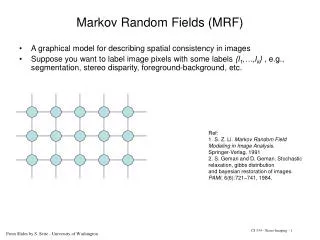
Markov Random Fields (MRF) A graphical model for describing spatial consistency in images Suppose you want to label image pixels with some labels {l1,…,lk} , e.g., segmentation, stereo disparity, foreground-background, etc. Ref: 1. S. Z. Li. Markov Random Field Modeling in Image Analysis. Springer-Verlag, 1991 2. S. Geman and D. Geman. Stochastic relaxation, gibbs distribution and bayesian restoration of images. PAMI, 6(6):721–741, 1984. CS 534 – Stereo Imaging - 1 From Slides by S. Seitz - University of Washington
Definition MRF Components: A set of sites: P={1,…,m} : each pixel is a site. Neighborhood for each pixel N={Np | p P} A set of random variables (random field), one for each site F={Fp | p P} Denotes the label at each pixel. Each random variable takes a value fp from the set of labels L={l1,…,lk} We have a joint event {F1=f1,…, Fm=fm} , or a configuration, abbreviated as F=f The joint prob. Of such configuration: Pr(F=f) or Pr(f) CS 534 – Stereo Imaging - 2 From Slides by S. Seitz - University of Washington
Definition MRF Components: Pr(fi) > 0 for all variables fi. Markov Property: Each Random variable depends on other RVs only through its neighbors. Pr(fp | fS-{p})=Pr (fp|fNp), p So, we need to define a neighborhood system: Np (neighbors for site p). No strict rules for neighborhood definition. Cliques for this neighborhood CS 534 – Stereo Imaging - 3 From Slides by S. Seitz - University of Washington
Definition MRF Components: The joint prob. of such configuration: Pr(F=f) or Pr(f) Markov Property: Each Random variable depends on other RVs only through its neighbors. Pr(fp | fS-{p})=Pr (fp|fNp), p So, we need to define a neighborhood system: Np (neighbors for site p) Hammersley-Clifford Theorem:Pr(f) exp(-C VC(f)) Sum over all cliques in the neighborhood system VCis clique potential We may decide 1. NOT to include all cliques in a neighborhood; or 2. Use different Vc for different cliques in the same neighborhood CS 534 – Stereo Imaging - 4 From Slides by S. Seitz - University of Washington
Optimal Configuration MRF Components: Hammersley-Clifford Theorem: Pr(f) exp(-C VC(f)) Consider MRF’s with arbitrary cliques among neighboring pixels Sum over all cliques in the neighborhood system VCis clique potential: prior probability that elements of the clique C have certain values Typical potential: Potts model: CS 534 – Stereo Imaging - 5 From Slides by S. Seitz - University of Washington
Optimal Configuration MRF Components: Hammersley-Clifford Theorem: Pr(f) exp(-C VC(f)) Consider MRF’s with clique potentials of pairs of neighboring pixels Most commonly used….very popular in vision. Energy function: There are two constraints to satisfy: • Data Constraint: Labeling should reflect the observation. • Smoothness constraint: Labeling should reflect spatial consistency (pixels close to each other are most likely to have similar labels). CS 534 – Stereo Imaging - 6
Probabilistic interpretation The problem is we are not observing the labels but we observe something else that depends on these labels with some noise (eg intensity or disparity) At each site we have an observation ip The observed value at each site depends on its label: the prob. of certain observed value given certain label at site p : g(ip,fp)=Pr(ip|Fp=fp) The overall observation prob. Given the labels: Pr(O|f) We need to infer about the labels given the observation Pr(f|O) Pr(O|f) Pr(f) CS 534 – Stereo Imaging - 7
Using MRFs How to model different problems? Given observations y, and the parameters of the MRF, how to infer the hidden variables, x? How to learn the parameters of the MRF?
Modeling image pixel labels as MRF MRF-based segmentation real image 1 label image Slides by R. Huang – Rutgers University
Modeling image pixel labels as MRF MRF-based segmentation real image 1 label image Slides by R. Huang – Rutgers University
Modeling image pixel labels as MRF MRF-based segmentation real image 1 label image
MRF-based segmentation Classifying image pixels into different regions under the constraint of both local observations and spatial relationships Probabilistic interpretation: region labels model param. image pixels Slides by R. Huang – Rutgers University
Model joint probability region labels model param. image pixels How did we factorize? image-label compatibility Function enforcing Data Constraint label-label compatibility Function enforcing Smoothness constraint label image local Observations neighboring label nodes Slides by R. Huang – Rutgers University
Probabilistic interpretation We need to infer about the labels given the observation Pr( f | O ) Pr(O|f ) Pr(f) MAP estimate of f should minimize the posterior energy Data (observation) term: Data Constraint Neighborhood term: Smoothness Constraint CS 534 – Stereo Imaging - 14
MRF-based segmentation EM algorithm E-Step: (Inference) M-Step: (learning) Applying and learning MRF Methods to be described. Pseduo-likelihood method. Slides by R. Huang – Rutgers University
Applying and learning MRF: Example Slides by R. Huang – Rutgers University
Inference in MRFs Inference in MRFs Classical: Gibbs sampling, simulated annealing Self study Iterated condtional modes (ICM) Also Self study State of the Art Graph cuts Belief propagation Linear Programming (not covered in this lecture) Tree-reweighted message passing (not covered in this lecture) Slides by R. Huang – Rutgers University
Gibbs sampling and simulated annealing Gibbs sampling: A way to generate random samples from a (potentially very complicated) probability distribution Simulated annealing: A schedule for modifying the probability distribution so that, at “zero temperature”, you draw samples only from the MAP solution. Simulated Annealing algorithm: x := x0; e := E(x) // Initial state, energy. k := 0 // Energy evaluation count. while k < kmax and e > emax // While time remains & not good enough: xn := neighbour(x) // Pick some neighbour. en := E(xn) // Compute its energy. if P(e, en, temp(k/kmax)) > random() then // Should we move to it? x := xn; e := en // Yes, change state. k := k + 1 // One more evaluation done return x // Return current solution Slides by R. Huang – Rutgers University
Gibbs sampling and simulated annealing cont. Simulated annealing as you gradually lower the “temperature” of the probability distribution ultimately giving zero probability to all but the MAP estimate. finds global MAP solution. takes forever. (Gibbs sampling is in the inner loop…) Slides by R. Huang – Rutgers University
Iterated conditional modes Start with an estimate of labeling x For each node xi: Condition on all the neighbors Find the label decreasing the energy function the most Repeat till convergence Fast Heavily depend on initialization, local minimum Described in: Winkler, 1995. Introduced by Besag in 1986. Slides by R. Huang – Rutgers University
Solving Energy Minimization with Graph Cuts • Many classes of Energy Minimization problems in Computer Vision can be reduced to Graph Cuts • Solve multiple-labels problems with binary decisions Yevgeny Doctor IP Seminar 2008, IDC
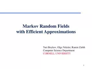
Approximate Energy Minimization • “Fast Approximate Energy Minimization via Graph Cuts.” Yuri Boykov, Olga Veksler, Ramin Zabih, 1999 • For two classes of interaction potentials V (Esmooth): • V is semi-metric on a label space L if for every : • V is metric on L if in addition, triangle inequality holds: • For example, truncated L2 distance and Potts Interaction Penalty are both metric. Yevgeny Doctor IP Seminar 2008, IDC
Solution for Semi-metric Class • Swap-Move algorithm: • 1. Start with an arbitrary labeling f • 2. Set success := 0 • 3. For each pair of labels • 3.1. Find f* = argmin E(f') among f' within one a-b swap of f • 3.2. If E(f*) < E(f), set f := f* and success := 1 • 4. If success = 1 goto 2 • 5. Return f • a-b swap: • In the new labeling f’, some pixels that were labeled a in f are now labeled b, and vice versa. Yevgeny Doctor IP Seminar 2008, IDC
Solve a-b swap step with Graph Cut • Graph: Fast Approximate Energy Minimization via Graph Cuts Yuri Boykov, Olga Veksler, Ramin Zabih, 1999 Yevgeny Doctor IP Seminar 2008, IDC
Solve a-b swap step with Graph Cut • Cut and Labeling: • Weights: Fast Approximate Energy Minimization via Graph Cuts Yuri Boykov, Olga Veksler, Ramin Zabih, 1999 Yevgeny Doctor IP Seminar 2008, IDC
Computing a multiway cut With two labels: classical min-cut problem Solvable by standard network flow algorithms polynomial time in theory, nearly linear in practice More than 2 labels: NP-hard But efficient approximation algorithms exist Within a factor of 2 of optimal Computes local minimum in a strong sense even very large moves will not improve the energy Yuri Boykov, Olga Veksler and Ramin Zabih, Fast Approximate Energy Minimization via Graph Cuts, International Conference on Computer Vision, September 1999. Basic idea reduce to a series of 2-way-cut sub-problems, using one of: swap move: pixels with label l1 can change to l2, and vice-versa expansion move: any pixel can change it’s label to l1 Slides by S. Seitz - University of Washington CS 534 – Stereo Imaging - 26
Belief propagation Message Passing (Original: Weiss & Freeman ‘01, faster: Felzenswalb & Huttenlocher ‘04) Send messages between neighbors. Messages estimate the cost (or Energy) of a configuration of a clique given all other cliques. s3 q q p = s2 s1 Messages are initialized to zero
Belief propagation Gathering belief After time T, the messages are combined to compute a belief. p3 p4 p2 q p1 Label with largest belief wins.
Inference in MRFs Loopy BP tractable, good approximate in network with loops Not guaranteed to converge, may oscillate infinitely.
Stereo as energy minimization Matching Cost Formulated as Energy: At pixel p = (x , y) “data” term penalizing bad matches “neighborhood term” encouraging spatial smoothness (truncated) Norm of the difference between labels at neighboring x, y. (also, truncated) From Slides by S. Seitz - University of Washington CS 534 – Stereo Imaging - 30
Stereo as a Graph cut Terminals (possible disparity labels) From Slides by Yuri Boykov, Olga Veksler, Ramin Zabih “Markov Random Fields with Efficient Approximations” – CVPR 98 CS 534 – Stereo Imaging - 31
Stereo as a graph problem [Boykov, 1999] Pixels edge weight d3 d2 d1 edge weight Labels (disparities) CS 534 – Stereo Imaging - 32 From Slides by S. Seitz - University of Washington
Graph definition Initial state Each pixel connected to it’s immediate neighbors Each disparity label connected to all of the pixels d3 d2 d1 From Slides by S. Seitz - University of Washington CS 534 – Stereo Imaging - 33
Stereo matching by graph cuts Graph Cut Delete enough edges so that each pixel is (transitively) connected to exactly one label node Cost of a cut: sum of deleted edge weights Finding min cost cut equivalent to finding global minimum of the energy function d3 d2 d1 From Slides by S. Seitz - University of Washington CS 534 – Stereo Imaging - 34
Motion estimation as energy minimization Matching Cost Formulated as Energy: At pixel p = (x , y) “data” term penalizing bad matches “neighborhood term” encouraging spatial smoothness (truncated) Norm of the difference between labels at neighboring x, y. (also, truncated) From Slides by S. Seitz - University of Washington CS 534 – Stereo Imaging - 35
Results with window search Window-based matching (best window size) Ground truth From Slides by S. Seitz - University of Washington CS 534 – Stereo Imaging - 36
Better methods exist... • State of the art method • Boykov et al., Fast Approximate Energy Minimization via Graph Cuts, • International Conference on Computer Vision, September 1999. Ground truth From Slides by S. Seitz - University of Washington CS 534 – Stereo Imaging - 37
GrabCut GrabCut Rother et al 2004 Magic Wand(198?) Intelligent ScissorsMortensen and Barrett (1995) User Input Result Regions Regions & Boundary Boundary Slides C Rother et al., Microsoft Research, Cambridge
Data Term R Foreground &Background Gaussian Mixture Model (typically 5-8 components) G Background D() is log-likelihood given the mixture model \Theta Slides C Rother et al., Microsoft Research, Cambridge
Smoothness term An object is a coherent set of pixels: Probability of a configuration: Iterate until convergence: 1. Compute a configuration given the mixture model. (E-Step) 2. Compute the model parameters given the configuration. (M-Step) Slides C Rother et al., Microsoft Research, Cambridge
Moderately simple examples … GrabCut completes automatically Slides C Rother et al., Microsoft Research, Cambridge
Difficult Examples Camouflage & Low Contrast Fine structure No telepathy Initial Rectangle InitialResult Slides C Rother et al., Microsoft Research, Cambridge