Graphical models, belief propagation, and Markov random fields

1. Graphical models, belief propagation, and Markov random fields

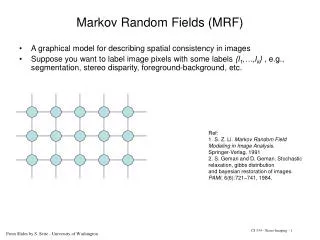
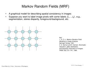
2. Markov Random Field (MRF) • Definition: A Markov random field, Markov network or undirected graphical model is a graphical model in which a set of random variables have a Markov property described by an undirected graph. A Markov random field is similar to a Bayesian network in its representation of dependencies. It can represent certain dependencies that a Bayesian network cannot (such as cyclic dependencies); on the other hand, it can't represent certain dependencies that a Bayesian network can (such as induced dependencies). The prototypical Markov random field is the Ising model; indeed, the Markov random field was introduced as the general setting for the Ising model From Wiki.

3. Problem solved by MRF • MRF is very popular and useful in both Computer Vision and Computer Graphic Areas. • Solve Discrete Labeling problem of graphical model • Segmentation, Stereo, Noise removal, etc. • Reading materials • Graphical models: Probabilistic inference, Michael I., Jordan and Yair Weiss • This topic itself can be another courses, I will cover this topic briefly related to our area. • You might not understand the mathematics, but you will learn how to use it. This is the goal of this class.

4. Things we want to be able to articulate in a spatial prior • Favor neighboring pixels having the same state (state, meaning: estimated depth, or group segment membership) • Favor neighboring nodes have compatible states (a patch at node i should fit well with selected patch at node j). • But encourage state changes to occur at certain places (like regions of high image gradient).

5. x1 x2 x3 y z Graphical models: tinker toys to build complex probability distributions • Circles represent random variables. • Lines represent statistical dependencies. • There is a corresponding equation that gives P(x1, x2, x3, y, z), but often it’s easier to understand things from the picture. • These tinker toys for probabilities let you build up, from simple, easy-to-understand pieces, complicated probability distributions involving many variables. http://mark.michaelis.net/weblog/2002/12/29/Tinker%20Toys%20Car.jpg

6. Steps in building and using graphical models • First, define the valuables, how many discrete labels in your valuables, eg. no. of depth label • Second, define function you want to optimize. Note the two common ways of framing the problem • In terms of probabilities. Multiply together component terms, which typically involve exponentials. • In terms of energies. The log of the probabilities. Typically add together the exponentiated terms from above. • The third step: optimize that function. For probabilities, take the mean or the max (or use some other “loss function”). For energies, take the min. • Find the set of label configuration that max/min the probabilities/energies.

7. Standard Form of MRF optimization argmaxxP(x|y) = argmaxx ÕF(xi,yi) ÕY(xi,xj) i i,j = argminx F*(xi,yi) +Y*(xi,xj) Hidden variable i i,j Data local observations Neighboring nodes Note:F* = log F Y * = log Y Data compatibility function Neighborhood compatibility function Our solution is a configuration of x that maximize/minimize the probabilities/energies

8. MRF - Graphical Model • Typical setup of MRF in image processing • Good News: Standard solver is available. • http://vision.middlebury.edu/MRF/ x,y are swapped in this figure

9. Method for solving MRF • Iterated conditional modes (ICM) • Described in: Winkler, 1995. Introduced by Besag in 1986 • Gibbs sampling, simulated annealing • Pros: finds global MAP solution. Cons: takes forever • Variational methods • TommiJaakkola’s tutorial on variational methods • http://www.ai.mit.edu/people/tommi/ • Example: mean field • State of the art (Standard) techniques in Computer Vision: • Belief propagation • Graph cuts

10. Comparison of graph cuts and belief propagation Comparison of Graph Cuts with Belief Propagation for Stereo, using Identical MRF Parameters, ICCV 2003. Marshall F. Tappen William T. Freeman

11. Ground truth, graph cuts, and belief propagation disparity solution energies

12. Graph cuts versus belief propagation • Graph cuts consistently gave slightly lower energy solutions for that stereo-problem MRF, although BP ran faster, although there is now a faster graph cuts implementation than what we used… • Conclusion: better results can be obtained with better defined Energies • Personally, I prefer Belief Propagation, and here are the reasons: • Works for any compatibility functions, not a restricted set like graph cuts. • I find it very intuitive. • Extensions: sum-product algorithm computes MMSE, and Generalized Belief Propagation gives you very accurate solutions, at a cost of time.

13. Belief propagation: the nosey neighbor rule “Given everything that I know, here’s what I think you should think” (Given the probabilities of my being in different states, and how my states relate to your states, here’s what I think the probabilities of your states should be)

14. Reminder: Standard Form of MRF optimization argmaxxP(x|y) = argmaxx ÕF(xi,yi) ÕY(xi,xj) i i,j = argminx F*(xi,yi) +Y*(xi,xj) Hidden variable i i,j Data local observations Neighboring nodes Note:F* = log F Y * = log Y Data compatibility function Neighborhood compatibility function Our solution is a configuration of x that maximize/minimize the probabilities/energies

15. Belief propagation messages A message: can be thought of as a set of weights on each of your possible states To send a message: Multiply together all the incoming messages, except from the node you’re sending to, then multiply by the compatibility matrix and marginalize over the sender’s states. = i j j i

16. Beliefs To find a node’s beliefs: Multiply together all the messages coming in to that node. j

17. x1 x2 x3 x1 x2 x3 Simple BP example y1 y3 This is defined based on your Prior This is defined based on the goodness-of-fit among observed date

18. x1 x2 x3 • To find the marginal probability for each variable, you can • Marginalize out the other variables of: • Or you can run belief propagation, (BP). BP redistributes the various partial sums, leading to a very efficient calculation. Simple BP example

19. Belief, and message updates j = i j i

20. Optimal solution in a chain or tree:Belief Propagation • “Do the right thing” Bayesian algorithm. • For Gaussian random variables over time: Kalman filter. • For hidden Markov models: forward/backward algorithm (and MAP variant is Viterbi). • Caution: For Cyclic Graph, there is no proof that BP converges, but we general believe it converges

21. References on BP and GBP • J. Pearl, 1985 • classic • Y. Weiss, NIPS 1998 • Inspires application of BP to vision • W. Freeman et al learning low-level vision, IJCV 1999 • Applications in super-resolution, motion, shading/paint discrimination • H. Shum et al, ECCV 2002 • Application to stereo • M. Wainwright, T. Jaakkola, A. Willsky • Reparameterization version • J. Yedidia, AAAI 2000 • The clearest place to read about BP and GBP.

22. Applications of MRF’s • Image Denoising • Stereo • Motion estimation • Labelling shading and reflectance • Many others…

23. Denoising • Each pixel is a node • Each pixel intensity is a stage of node Input Gau. Filter Median Filter MRF Ground Truth

24. Stereo • Each depth is stage of node

25. Motion estimation • Each motion direction is a stage of node • Segmentation information can also be included into Prior From Zitnick et al. ICCV’05

26. Intrinsic Image Estimation Input Image Reflectance Image Without Propagation Reflectance Image With Propagation Tappen et al. NIPS’02

28. Image Segmentation • Lazy snapping, etc. • Each node stage is the segmentation label

29. Texture Synthesis • Graphcut Textures, Siggraph’03

30. Super resolution • Learning low level vision, IJCV’00

31. Image Completion • Image Completion with Structure Propagation, Siggraph’05

32. Summary • Solve Discrete Labelling / Graph Partitioning problems • MRF is useful, many applications in vision and graphics, it’s also useful in other areas • To use MRF • define your data term from observation • define your neighbor term from Priors • Standard solver (support both BP and Graphcut) is available: http://vision.middlebury.edu/MRF/