Markov Random Fields and Gibbs Measures
Learn about Markov random fields, Gibbs measures, potential functions, Hammersley-Clifford theorem, Ising model, simulated fields, Gaussian conditional autoregressive models, spatial covariance, and more.


Markov Random Fields and Gibbs Measures
E N D
Presentation Transcript
The Markov property Discrete time: A time symmetric version: A more general version: Let A be a set of indices >k, B a set of indices <k. Then These are all equivalent.
On a spatial grid Let i be the neighbors of the location i. The Markov assumption is Equivalently for The pi are called local characteristics. They are stationary if pi = p. A potential assigns a number VA(z) to every subconfiguration zA of a configuration z. (There are lots of them!)
Graphical models Neighbors are nodes connected with edges. Given 2, 1 and 4 are independent. 2 4 1 5 3
Gibbs measure The energy U corresponding to a potential V is . The corresponding Gibbs measure is where is called the partition function.
Nearest neighbor potentials A set of points is a clique if all its members are neighbours. A potential is a nearest neighbor potential if VA(z)=0 whenever A is not a clique.
Markov random field Any nearest neighbour potential induces a Markov random field: where z’ agrees with z except possibly at i, so VC(z)=VC(z’) for any C not including i.
The Hammersley-Clifford theorem Assume P(z)>0 for all z. Then P is a MRF on a (finite) graph with respect to a neighbourhood system iff P is a Gibbs measure corresponding to a nearest neighbour potential. Does a given nn potential correspond to a unique P?
The Ising model Model for ferromagnetic spin (values +1 or -1). Stationary nn pair potential V(i,j)=V(j,i); V(i,i)=V(0,0)=v0; V(0,eN)=V(0,eE)=v1. so where
Interpretation v0 is related to the external magnetic field (if it is strong the field will tend to have the same sign as the external field) v1 corresponds to inverse temperature (in Kelvins), so will be large for low temperatures.
Phase transition At very low temperature there is a tendency for spontaneous magnetization. For the Ising model, the boundary conditions can affect the distribution of x0. In fact, there is a critical temperature (or value of v1) such that for temperatures below this the boundary conditions are felt. Thus there can be different probabilities at the origin depending on the values on an arbitrary distant boundary!
Tomato disease Data on spotted wilt from the Waite Institute 1929. 16 plots in 4x4 Latin square, each 6 rows with 15 plants each. Occurrence of the viral disease 23 days after planting.
Exponential tilting Simulate from the model u and estimate the expectation by an average.
Fitting the tomato data t0 = - 834 t1=2266 Condition on boundary and simulate 100,000 draws from u=(0,0.5). Mle The simulated values of t0 are half positive and half negative (phase transition).
The auto-models Let Q(x)=log(P(x)/P(0)). Besag’s auto-models are defined by When and Gi(zi)=iwe get the autologistic model When and ij≤0 we get the auto-Poisson model
Coding schemes In order to estimate parameters, it can be easier to not use all the data. Besag suggested a coding scheme in which one only uses data at points which are conditionally independent (given all the other data):
Pseudolikelihood Another approximate approach is to write down a function of the data which is the product of the , I.e., acting as if the neighborhoods of each point were independent. This as an estimating equation, but not an optimal one. In fact, in cases of high dependence it tends to be biased.
Recall the Gaussian formula If then Let be the precision matrix. Then the conditional precision matrix is
Gaussian MRFs We want a setup in which whenever i and j are not neighbors. Using the Gaussian formula we see that the condition is met iff Qij = 0. Typically the precision matrix of a GMRF is sparse where the covariance is not. This allows fast computation of likelihoods, simulation etc.
An AR(1) process Let . The lag k autocorrelation is |k|. The precision matrix has Qij = if |I-j|=1, Q11=Qnn=1 and Qii=1+2 elsewhere. Thus has n2 non-zero elements, while Q has n+2(n-1)=3n-2 non-zero elements. Using the Gaussian formula we see that
Conditional autoregression Suppose that This is called a Gaussian conditional autoregressive model. WLOG i=0. If also these conditional distributions correspond to a multivariate joint Gaussian distribution, mean 0 and precision Q with Qii=i and Qij= -iij, provided Q is positive definite. If the ij are nonzero only when i~j we have a GMRF.
Likelihood calculation The Cholesky decomposition of a pd square matrix A is a lower triangular matrix L such that A=LLT. To solve Ay = b first solve Lv = b (forward substitution), then LTy = v (backward substitution). If a precision matrix Q = LLT, log det(Q) = 2 . The quadratic form in the likelihood is wTu where u=Qw and w=(z-). Note that
Simulation Let x ~ N(0,I), solve LTv = x and set z = + v. Then E(z) = and Var(z) = (LT)-1IL-1= (LLT)-1 = Q-1.
Spatial covariance Whittle (1963) noted that the solution to the stochastic differential equation has covariance function Rue and Tjelmeland (2003) show that one can approximate a Gaussian random field on a grid by a GMRF.
Unequal spacing Lindgren and Rue show how one can use finite element methods to approximate the solution to the sde (even on a manifold like a sphere) on a triangulization on a set of possibly unequally spaced points.
Precipitation in the Sahel The African Sahel region (south of Sahara) suffered severe drought in the 70s through 90s. There is recent evidence of recovery. Data from GHCN at 550 stations 1982-1996 (monthly, aggregated to annual).
Model Precipitation is determined by a latent (hidden) process, modelled as a Gaussian process on the sphere. This is approximated by a GMRF Z(si,tj)on a discrete number of points:
Details Y(s,t) = P(s,t)1/3(1-0.13P(s,t)1/3) = Z(s,t)+ Mean is a linear combination of basis functions (B-splines). Temporal structure is AR(1). Fitting by MCMC.
Reserved data Model check by reserving 10 stations.