Markov Random Fields
Markov Random Fields. Presented by: Vladan Radosavljevic. Outline. Intuition Simple Example Theory Simple Example - Revisited Application Summary References. Intuition. Simple example Observation noisy image pixel values are -1 or +1 Objective recover noise free image.


Markov Random Fields
E N D
Presentation Transcript
Markov Random Fields Presented by: Vladan Radosavljevic
Outline • Intuition • Simple Example • Theory • Simple Example - Revisited • Application • Summary • References
Intuition • Simple example • Observation • noisy image • pixel values are -1 or +1 • Objective • recover noise free image
Intuition • An idea • Represent pixels as random variables • y - observed variable • x - hidden variable x and y are binary variables (-1 or +1) • Question: • Is there any relation among those variables?
Intuition • Building a model • Values of observed and original pixels should be correlated (small level of noise) - make connections! • Values of neighboring pixels should be correlated (large homogeneous areas, objects) - make connections! Final model
Intuition • Why do we need a model? • y is given, x has to be find • The objective is to find an image x that maximizes p(x|y) • Use model • penalize connected pairs in the model that have opposite sign as they are not correlated • Assume distribution p(x,y) ~ exp(-E) E = over all pairs of connected nodes • If xi and xj have the same sign, the probability will be higher • The same holds for x and y
Intuition • How to find an image x which maximizes probability p(x|y)? • Assume x=y • Take a node xi at time and evaluate E for xi=+1and xi=-1 • Set xi to the value that has lowest E (highest probability) • Iterate through all nodes until convergence • This method finds local optimum
Intuition • Result
Theory • Graphical models – a general framework for representing and manipulating joint distributions defined over sets of random variables • Each variable is associated with a node in a graph • Edges in the graph represent dependencies between random variables • Directed graphs: represent causative relationships (Bayesian Networks) • Undirected graphs: represent correlative relationships (Markov Random Fields) • Representational aspect: efficiently represent complex independence relations • Computational aspect: efficiently infer information about data using independence relations
Theory • Recall • If there are M variables in the model each having K possible states, straight forward inference algorithm will be exponential in the size of the model (KM) • However, inference algorithms (whether computing distributions, expectations etc.) can use structure in the graph for the purposes of efficient computation
Theory • How to use information from the structure? • Markov property: If all paths that connect nodes in set A to nodes in set B pass through nodes in set C, then we say that A and B are conditionally independent given C: • p(A,B|C) = p(A|C)p(B|C) • The main idea is to factorize joint probability, then use sum and product rules for efficient computation
Theory • General factorization • If two nodes xiand xkare not connected, then they have to be conditionally independent given all other nodes • There is no link between those two nodes and all other links pass through nodes that are observed • This can be expressed as • Therefore, joint distribution must be factorized such that unconnected nodes do not appear in the same factor • This leads to the concept of clique: a subset of nodes such that all pairs of nodes in the subset are connected • The factors are defined as functions on the all possible cliques
Theory • Example • Factorization where : potential function on the clique C Z : partition function
Theory • Since potential functions have to be positive we can define them as: • (there is also a theorem that proofs correspondence of this distribution and Markov Random Fields, E is energy function) • Recall • E =
Theory • Why is this useful? • Inference algorithms can take an advantage of such representation to significantly increase computational efficiency • Example, inference on a chain • To find marginal distribution ~ KN
Theory • If we rearrange the order of summations and multiplications ~ NK2
Summary • Advantages • Graphical representation • Computational efficiency • Disadvantages • Parameter estimation • How to define a model? • Computing probability is sometimes difficult
References • [1] Alexander T. Ihler, Sergey Kirshner, Michael Ghilc, Andrew W. Robertson and Padhraic Smyth “Graphical models for statistical inference and data assimilation”, Physica D: Nonlinear Phenomena, Volume 230, Issues 1-2, June 2007, Pages 72-87