4054 Machine Vision Markov Random Fields
4054 Machine Vision Markov Random Fields. Dr. Simon Prince Dept. Computer Science University College London. http://www.cs.ucl.ac.uk/s.prince/4054.htm. Markov Random Fields. Dense stereo matching Incorporating smoothness constraints Markov random fields MCMC methods for MRFs


4054 Machine Vision Markov Random Fields
E N D
Presentation Transcript
4054 Machine VisionMarkov Random Fields Dr. Simon Prince Dept. Computer Science University College London http://www.cs.ucl.ac.uk/s.prince/4054.htm
Markov Random Fields • Dense stereo matching • Incorporating smoothness constraints • Markov random fields • MCMC methods for MRFs • Inference in MRFs with graph cuts • Applications of graph cuts • Multi-label energies
Markov Random Fields 1. Dense Stereo Matching
Dense Stereo Vision Image 1 Image 2 Disparity • Problem: • for each pixel in image 1, find matching pixel in image 2 • images rectified so offset only in horizontal direction • offset is termed disparity
Probabilistic Formulation Definitions: Grey value of pixel at pixel i,j in the first image Grey value of pixel at pixel i,j in the second image x11 x33 x43 x23 Hidden disparity label at pixel i,j in the first image Takes values from 0 to K x12 x32 x42 x22 x11 x31 x41 x21 Generative Approach:Associate discrete hidden variable l indicating disparity with each pixel x in the first image. Describe dependence of x on l, Pr(x|l) Define prior over hidden label, l Use Bayes’ rule to calculate Pr(l|x) Choose MAP solution arg max Pr(l|x) l11 l33 l43 l23 l12 l32 l42 l22 l11 l31 l41 l21 l
Probabilistic Formulation 1. Describe dependence of x on l, Pr(x|l) : Gaussian corruption of offset pixel in y 2. Define prior over hidden label l 3. Use Bayes’ rule to calculate Pr(l|x)
Probabilistic Formulation: Results 4. Choose MAP solution arg max Pr(l|x) l MAP Solution Ground Truth Solution is (unsurprisingly) very noisy – the disparity is often estimated wrongly How could we improve things?
Markov Random Fields 2. Incorporating Smoothness Constraints
The need for smoothing Stereo Vision Background Subtraction • Each of these results could be improved by adding the following prior knowledge: • We expect the label field to be smooth: • neighbouring disparities are usually similar • skin regions are usually contiguous in space • occlusion of the background is usually contiguous in space Colour Segmentation
Three models for smoothing l11 l11 l11 l33 l33 l33 l43 l43 l43 l23 l23 l23 Hidden labels l12 l12 l12 l32 l32 l32 l42 l42 l42 l22 l22 l22 l11 l11 l11 l31 l31 l31 l41 l41 l41 l21 l21 l21 x11 x11 x11 x33 x33 x33 x43 x43 x43 x23 x23 x23 x12 x12 x12 x32 x32 x32 x42 x42 x42 x22 x22 x22 Observed image x11 x11 x11 x31 x31 x31 x41 x41 x41 x21 x21 x21 Each node connected to all neighbours Label nodes connected along rows. Label nodes connected in a tree Connections: Markov Random Field Markov Chain Markov Tree (?) Model: Dynamic Programming Dynamic Programming on a tree Gibbs sampling, graph cuts Algorithm:
Smoothing Along Rows MAP solution is given by the labels li that maximize the numerator Previously, the labels were independent, so we could find the MAP solution at every pixel. However, they are now all connected. For any hypothesized set of disparity labels li for the line, we can calculate the RHS. However, there are too many possible disparity configurations to search exhaustively e.g. 21 possible disparities, J=640 pixels gives 21640 configurations
Smoothing Along Rows Key idea: some conjunctions of neighbouring labels are more likely than others. In particular: Where prob c1 for disparity staying the same < prob c2 for disparity change of one < prob c3 for disparity change of more than one Solution: use Bayes’ rule to establish posterior over labels
Smoothing Along Rows Goal: Consider the terms in the right hand side separately: Data likelihoods are independent from each other, so this term factorizes. What about the prior? The prior also factorizes. We can exploit this!
Dynamic Programming • We can equivalently maximize the logarithm - monotonic transformation, so extrema are in the same positions. • Alternatively, we could minimize the negative logarithm • Now minimizing something of the form Where Aj = -log Pr(xi,j|y,s,li,j) and Bj,j-1 = -logPr(li,j|li,j-1)
x1 x2 x3 x4 x5 x6 DP Problem Overview • B4,5 • A2(1) • B4,5 • A2(2) k=1 • B4,5 • B4,5 • A2(3) k=2 • B4,5 • A2(4) k=3 Disparity, k in pixels • A2(5) k=4 k=5 Nb. Nodes do not have same meaning as in graphical models! GOAL: find minimum cost path from left to right. Position in First Image Assume const Node costs Link costs
x1 x2 x3 x4 x5 x6 DP Worked Example 2 1 6 3 6 1 k=1 1 5 1 3 6 3 k=2 4 2 2 6 6 2 k=3 Disparity, k in pixels 5 0 5 1 6 2 k=4 2 2 5 8 1 9 k=5 Position in First Image Node costs indicated in red. Link costs: 0 for constant disparity 2 to change disparity by 1 100 to change disparity by more than one
x1 x2 x3 x4 x5 x6 DP Worked Example 1 6 3 6 1 k=1 2 5 1 3 6 3 k=2 1 2 2 6 6 2 k=3 Disparity, k in pixels 4 0 5 1 6 2 k=4 5 2 5 8 1 9 k=5 2 Position in First Image Start from left. At each stage fill in nodes with cheapest possible path to this point so far by any route. For the first node this will be just the first node costs
x1 x2 x3 x4 x5 x6 DP Worked Example 1 6 3 6 1 k=1 3 2 5 1 3 6 3 k=2 1 2 2 6 6 2 k=3 Disparity, k in pixels 4 0 5 1 6 2 k=4 5 2 5 8 1 9 k=5 2 Position in First Image Consider node at x=2,k=1. Consider all possible routes to reach this node – cheapest way is to go straight across from x=1,k=1. Total cost = 2 (cost at x=1,k=1) + 0 (link cost) +1 (cost at x=2,k=1) = 3
x1 x2 x3 x4 x5 x6 DP Worked Example 1 6 3 6 1 k=1 3 2 5 1 3 6 3 k=2 6 1 2 2 6 6 2 k=3 Disparity, k in pixels 4 0 5 1 6 2 k=4 5 2 5 8 1 9 k=5 2 Position in First Image Consider node at x=2,k=2. Consider all possible routes to reach this node – cheapest way is to go straight across from x=1,k=2. Total cost = 1 (cost at x=1,k=2) + 0 (link cost) +5 (cost at x=2,k=2) = 6
x1 x2 x3 x4 x5 x6 DP Worked Example 1 6 3 6 1 k=1 3 3 2 5 1 3 6 3 k=2 6 1 2 2 6 6 2 k=3 Disparity, k in pixels 5 4 0 5 1 6 2 k=4 5 2 5 8 1 9 k=5 2 Position in First Image Consider node at x=2,k=3. Consider all possible routes to reach this node – cheapest way is to come down from x=1,k=2. Total cost = 1 (cost at x=1,k=2) + 2 (link cost) +2 (cost at x=2,k=3) = 5
x1 x2 x3 x4 x5 x6 DP Worked Example 6 3 6 1 k=1 9 3 2 1 3 6 3 k=2 6 1 2 6 6 2 k=3 Disparity, k in pixels 5 4 5 1 6 2 k=4 5 5 5 8 1 9 k=5 4 2 Position in First Image Each time we update a node, remember the route by which we got there. We need to store one link entering each node. Now repeat this procedure for position x =3,k=1.
x1 x2 x3 x4 x5 x6 DP Worked Example 6 3 1 k=1 3 9 2 3 6 3 k=2 6 6 1 6 6 2 k=3 Disparity, k in pixels 5 7 4 1 6 2 k=4 5 10 5 8 1 9 k=5 4 9 2 Position in First Image Situation after considering all routes to x=3.
x1 x2 x3 x4 x5 x6 DP Worked Example k=1 3 9 9 15 18 2 k=2 6 6 9 15 18 1 k=3 Disparity, k in pixels 5 7 9 15 21 4 k=4 5 10 10 16 17 5 k=5 4 9 13 13 21 2 Position in First Image Situation after completing the entire row of pixels
x1 x2 x3 x4 x5 x6 DP Worked Example k=1 3 9 9 15 18 2 k=2 6 6 9 15 18 1 k=3 Disparity, k in pixels 5 7 9 15 21 4 k=4 5 10 10 16 17 5 k=5 4 9 13 13 21 2 Position in First Image Identify the minimum cumulative cost on the right. This is the minimum possible cost for passing from left to right.
x1 x2 x3 x4 x5 x6 DP Worked Example k=1 3 9 9 15 18 2 k=2 6 6 9 15 18 1 k=3 Disparity, k in pixels 5 7 9 15 21 4 k=4 5 10 10 16 17 5 k=5 4 9 13 13 21 2 Position in First Image Trace back the patch by which the minimum cost has been achieved.
Dynamic Programming Results No smoothing Increasing smoothing Most smoothing Increasing smoothing
Dynamic Programming Complexity • Computational complexity of dynamic programming much less than the original brute force search: • Assume: • J pixels • K disparity values • Brute force search: O(KJ) • Dynamic Programming? • For each of J pixels • Consider each of K disparity levels • Consider K possible paths into each level • Complexity = O(JK2) J pixels ... 3 3 2 ... 1 ... K disparity values 4 ... 5 ... 2
Three models for smoothing l11 l11 l11 l33 l33 l33 l43 l43 l43 l23 l23 l23 Hidden labels l12 l12 l12 l32 l32 l32 l42 l42 l42 l22 l22 l22 l11 l11 l11 l31 l31 l31 l41 l41 l41 l21 l21 l21 x11 x11 x11 x33 x33 x33 x43 x43 x43 x23 x23 x23 x12 x12 x12 x32 x32 x32 x42 x42 x42 x22 x22 x22 Observed image x11 x11 x11 x31 x31 x31 x41 x41 x41 x21 x21 x21 Each node connected to all neighbours Label nodes connected along rows. Label nodes connected in a tree Connections: Markov Random Field Markov Chain Markov Tree (?) Model: Dynamic Programming Dynamic Programming on a tree Gibbs sampling, graph cuts Algorithm:
Tree Structure PROBLEM: Solving independently for each line using dynamic programming results in characteristic ‘streaky’ solution SOLUTION: Find a way to connect all of the nodes? 2. Assign importance to each link 3. Prune links until no loops left (a tree) 1. Start with fully connected grid
Advantage of Tree Structure • Prior over labels still factorizes • Can still perform dynamic programming • Start from leaves and move up tree • Efficiently get exactly correct answer • Suggested for stereo by Veksler (2005) • How do we decide which links to keep and which to throw away? • Not so important to have smoothness where there are large changes in intensity: • May be an edge anyway • More reliable info for matching here
Markov Random Fields 3. Markov Random Fields
Three models for smoothing l11 l11 l11 l33 l33 l33 l43 l43 l43 l23 l23 l23 Hidden labels l12 l12 l12 l32 l32 l32 l42 l42 l42 l22 l22 l22 l11 l11 l11 l31 l31 l31 l41 l41 l41 l21 l21 l21 x11 x11 x11 x33 x33 x33 x43 x43 x43 x23 x23 x23 x12 x12 x12 x32 x32 x32 x42 x42 x42 x22 x22 x22 Observed image x11 x11 x11 x31 x31 x31 x41 x41 x41 x21 x21 x21 Each node connected to all neighbours Label nodes connected along rows. Label nodes connected in a tree Connections: Markov Random Field Markov Chain Markov Tree (?) Model: Dynamic Programming Dynamic Programming on a tree Gibbs sampling, graph cuts Algorithm:
What is a Markov random field? • our goal is to specify a prior over labellings • we consider binary case l = {1,2} • if P pixels in image then 2P possible label fields • want to make some of these more likely than others CRITERION: smoothness - favour solutions where 1’s are next to 1’s and 2’s tend to be next to 2’s. Markov as probability relations defined only between neighbours. Field as 2d grid of labels Less likely solution More likely solution
Markov random field a set of sites S = S1...SP . These will be the P pixels. a neighbourhood system .. This defines the extent of the local probabilistic connections between sites. a set of random variables . These are unknown binary labels indicating foreground or background. Definition of a Markov random field Just a restatement of what we saw in the graphical model...
Hammersley-Clifford Theorem The Hammersley-Clifford theorem states that a system that obeys the MRF definition can be written as a Gibbs’ distribution: This is not obvious! U= cost for MRF – as U increases, probability decreases. T= temperature (usually 1) Z = partition function, unknowable normalization constant
Clique Potentials What is in U(l)? It is the sum of clique potentials, Vc(l). • What are the clique potentials? • clique is a minimal group of connected pixels • in this example, cliques are pairs of neighbouring pixels. • pairs are ordered, so two clique potentials per link. • What form do they take? • a table indicating costs for adjacent pairs of node values • for smoothness w21, w12 > w11,w22 ln
Incorporating unary prior term • so far, only have a prior over labels favouring smoothness. • most likely images are all uniform l=1 or l=2 • can also incorporate a per pixel bias Pr(li) towards li=1 or li=2 • Examples • more likely to be background than foreground • More likely to see skin pixels in middle of image
MAP Estimation with MRFs • Having defined prior, can combine with a data term • Use Bayes’ rule for MAP inference • Now the posterior label field must: • agree with the data • obey the smoothness prior • Writing out in full : • unknown constant doesn’t matter for MAP estimate
MAP Estimation with MRFs For any label field l, can calculate the posterior (up to unknown but constant scaling factor) using: How do we find the labels l that maximize this expression? Brute force won’t work! VGA: 2640x480 possible label fields. Q. Is it even possible to find the MAP estimate? • We will consider two types of solution: • Approximate : Markov Chain Monte Carlo methods • Exact : graph cuts
Markov Random Fields 4. MCMC Methods for MRFs
MCMC Methods • KEY IDEA: • randomly draw many samples from the posterior distribution • most probable sample MAP estimate • PROBLEM: • drawing samples from high dimensional p.d.f. is hard. • want samples mainly from regions of high probability • don't know where these regions are • cannot evaluate all of the states to find out • SOLUTION: • Markov chain Monte Carlo (MCMC) methods designed to sample from complex probability distributions • generate a series (CHAIN) of samples from the distribution, • each sample depends directly on the previous one. (MARKOV) • sampling stochastic (MONTE-CARLO) • after running for a long time – get samples as required
Gibbs Sampling • Key idea: • Choose one dimension (label) at a time. • Calculate posterior probability distribution for this label assuming all the others are fixed • Sample from this one dimensional distribution • Update label with this sample • Notice that unknown constant cancels top and bottom
Example – Sampling from MRF prior Run 1 Run 2 Run 3 • Started with random binary labels • 2,000,000 rounds of Gibbs sampling • prior favours solutions that are locally smooth • no data term here or bias towards either label
Example – Colour Segmentation (B) (C) (A) (D) (E) Iter 0 Iter 4,000,000 Iter 8,000,000 Iter 12,000,000 Iter 16,000,000 (F) (G) (H) (I) (J) Iter 20,000,000 Iter 24,000,000 Iter 28,000,000 Iter 32,000,000 Iter 36,000,000
MCMC Summary • ADVANTAGES: • Very simple to implement • Very general: works for binary-label, multi-label, continuous label distributions • DISADVANTAGES: • Not guaranteed to get correct answer in finite time • Don’t know if we have the correct answer • Computationally expensive • Now introduce algorithm to find exact answer in binary case
Markov Random Fields 5. Inference in MRFs with graph cuts
Graph Cuts GOAL: Calculate exact MAP solution for binary MRF Three steps: Reformulate the maximization of the posterior probability function in terms of energy minimization. Express this minimization in terms of finding the minimum cut on a graph Find the minimum cut by solving an equivalent problem - finding the maximum flow from source to sink in a graph.
Energy Minimization GOAL: To re-express MAP estimation as energy minimization Take logarithm – does not effect position of maximum This is equivalent to minimizing an expression of the form: and : is cost for lm,ln where :