Markov Random Fields with Efficient Approximations
Markov Random Fields with Efficient Approximations. Yuri Boykov, Olga Veksler, Ramin Zabih Computer Science Department CORNELL UNIVERSITY. Introduction. MAP-MRF approach (Maximum Aposteriori Probability estimation of MRF)

Markov Random Fields with Efficient Approximations
E N D
Presentation Transcript
Markov Random Fields with Efficient Approximations Yuri Boykov, Olga Veksler, Ramin Zabih Computer Science Department CORNELL UNIVERSITY
Introduction MAP-MRF approach (Maximum Aposteriori Probability estimation of MRF) • Bayesian framework suitable for problems in Computer Vision (Geman and Geman, 1984) • Problem: High computational cost. Standard methods (simulated annealing) are very slow.
Outline of the talk • Models where MAP-MRF estimation is equivalent to min-cut problem on a graph • generalized Potts model • linear clique potential model • Efficient methods for solving the corresponding graph problems • Experimental results • stereo, image restoration
- disparity at pixel p - configuration MRF framework in the context of stereo • image pixels (vertices) • neighborhood relationships (n-links) MRF defining property: Hammersley-Clifford Theorem:
Observed data Bayes rule Prior (MRF model) Likelihood function (sensor noise) MAP estimation of MRF configuration
Find that minimizes the Posterior Energy Function : Smoothness term (MRF prior) Data term (sensor noise) Energy minimization
Clique potential Penalty for discontinuity at (p,q) Energy function Generalized Potts model
Disparity configurations minimizing energy E( f ): Static clues - selecting Stereo Image: White Rectangle in front of the black background
Terminals (possible disparity labels) Cost of n-link Cost of t-link Minimization of E(f) via graph cuts p-vertices (pixels)
Graph G = <V,E> Graph G(C) = <V, E-C > • A multiway cut Cyields some disparity configuration Multiway cut verticesV = pixels + terminals Remove a subset of edgesC edges E = n-links + t-links • Cis a multiway cut if terminals are separated inG(C)
Main Result(generalized Potts model) • Under some technical conditions on the multiway min-cut C on G gives___ that minimizes E( f ) - the posterior energy function for the generalized Potts model. • Multiway cut Problem: find minimum cost multiway cut C graph G
Solving multiway cut problem • Case of two terminals: • max-flow algorithm (Ford, Fulkerson 1964) • polinomial time (almost linear in practice). • NP-complete if the number of labels >2 • (Dahlhauset al., 1992) • Efficient approximation algorithms that are optimal within a factor of 2
Our algorithm Initialize at arbitrary multiway cut C 1. Choose a pair of terminals 2. Consider connected pixels
Our algorithm Initialize at arbitrary multiway cut C 1. Choose a pair of terminals 2. Consider connected pixels 3. Reallocate pixels between two terminals by running max-flow algorithm
Our algorithm Initialize at arbitrary multiway cut C 1. Choose a pair of terminals 2. Consider connected pixels 3. Reallocate pixels between two terminals by running max-flow algorithm 4. New multiway cut C’is obtained Iterate until no pair of terminals improves the cost of the cut
Experimental results (generalized Potts model) • Extensive benchmarking on synthetic images and on real imagery with dense ground truth • From University of Tsukuba • Comparisons with other algorithms
Correlation Multiway cut Synthetic example Image
Real imagery with ground truth Ground truth Our results
Comparative results: normalized correlation Gross errors Data
Related work (generalized Potts model) • Greig et al., 1986 is a special case of our method (two labels) • Two solutions with sensor noise (function g) highly restricted • Ferrari et al., 1995, 1997
Clique potential Penalty for discontinuity at (p,q) Energy function Linear clique potential model
cut C Cost of n-link Cost of t-link {p,q} part of graph a cut C yields some configuration Minimization of via graph cuts
Main Result(linear clique potential model) • Under some technical conditions on the min-cut C on gives that minimizes - the posterior energy function for the linear clique potential model.
Related work (linear clique potential model) • Ishikawa and Geiger, 1998 • earlier independently obtained a very similar result on a directed graph • Roy and Cox, 1998 • undirected graph with the same structure • no optimality properties since edge weights are not theoretically justified
Experimental results (linear clique potential model) • Benchmarking on real imagery with dense ground truth • From University of Tsukuba • Image restoration of synthetic data
Generalized Potts model Linear clique potential model ground truth Ground truth stereo image
Generalized Potts model Linear clique potential model Noisy diamond image Image restoration