Chi-Square Test
Chi-Square Test. A fundamental problem is genetics is determining whether the experimentally determined data fits the results expected from theory (i.e. Mendel’s laws as expressed in the Punnett square).

Chi-Square Test
E N D
Presentation Transcript
Chi-Square Test • A fundamental problem is genetics is determining whether the experimentally determined data fits the results expected from theory (i.e. Mendel’s laws as expressed in the Punnett square). • How can you tell if an observed set of offspring counts is legitimately the result of a given underlying simple ratio? For example, you do a cross and see 290 purple flowers and 110 white flowers in the offspring. This is pretty close to a 3/4 : 1/4 ratio, but how do you formally define "pretty close"? What about 250:150?
Goodness of Fit • Mendel has no way of solving this problem. Shortly after the rediscovery of his work in 1900, Karl Pearson and R.A. Fisher developed the “chi-square” test for this purpose. • The chi-square test is a “goodness of fit” test: it answers the question of how well do experimental data fit expectations. • We start with a theory for how the offspring will be distributed: the “null hypothesis”. We will discuss the offspring of a self-pollination of a heterozygote. The null hypothesis is that the offspring will appear in a ratio of 3/4 dominant to 1/4 recessive.
Formula • First determine the number of each phenotype that have been observed and how many would be expected given basic genetic theory. • Then calculate the chi-square statistic using this formula. You need to memorize the formula! • The “Χ” is the Greek letter chi; the “∑” is a sigma; it means to sum the following terms for all phenotypes. “obs” is the number of individuals of the given phenotype observed; “exp” is the number of that phenotype expected from the null hypothesis. • Note that you must use the number of individuals, the counts, and NOT proportions, ratios, or frequencies.
Example • As an example, you count F2 offspring, and get 290 purple and 110 white flowers. This is a total of 400 (290 + 110) offspring. • We expect a 3/4 : 1/4 ratio. We need to calculate the expected numbers (you MUST use the numbers of offspring, NOT the proportion!!!); this is done by multiplying the total offspring by the expected proportions. This we expect 400 * 3/4 = 300 purple, and 400 * 1/4 = 100 white. • Thus, for purple, obs = 290 and exp = 300. For white, obs = 110 and exp = 100. • Now it's just a matter of plugging into the formula: 2 = (290 - 300)2 / 300 + (110 - 100)2 / 100 = (-10)2 / 300 + (10)2 / 100 = 100 / 300 + 100 / 100 = 0.333 + 1.000 = 1.333. • This is our chi-square value: now we need to see what it means and how to use it.
Chi-Square Distribution • Although the chi-square distribution can be derived through math theory, we can also get it experimentally: • Let's say we do the same experiment 1000 times, do the same self-pollination of a Pp heterozygote, which should give the 3/4 : 1/4 ratio. For each experiment we calculate the chi-square value, them plot them all on a graph. • The x-axis is the chi-square value calculated from the formula. The y-axis is the number of individual experiments that got that chi-square value.
Chi-Square Distribution, p. 2 • You see that there is a range here: if the results were perfect you get a chi-square value of 0 (because obs = exp). This rarely happens: most experiments give a small chi-square value (the hump in the graph). • Note that all the values are greater than 0: that's because we squared the (obs - exp) term: squaring always gives a non-negative number. • Sometimes you get really wild results, with obs very different from exp: the long tail on the graph. Really odd things occasionally do happen by chance alone (for instance, you might win the lottery).
The Critical Question • how do you tell a really odd but correct result from a WRONG result? The graph is what happens with real experiments: most of the time the results fit expectations pretty well, but occasionally very skewed distributions of data occur even though you performed the experiment correctly, based on the correct theory, • The simple answer is: you can never tell for certain that a given result is “wrong”, that the result you got was completely impossible based on the theory you used. All we can do is determine whether a given result is likely or unlikely. • Key point: There are 2 ways of getting a high chi-square value: an unusual result from the correct theory, or a result from the wrong theory. These are indistinguishable; because of this fact, statistics is never able to discriminate between true and false with 100% certainty. • Using the example here, how can you tell if your 290: 110 offspring ratio really fits a 3/4 : 1/4 ratio (as expected from selfing a heterozygote) or whether it was the result of a mistake or accident-- a 1/2 : 1/2 ratio from a backcross for example? You can’t be certain, but you can at least determine whether your result is reasonable.
Reasonable • What is a “reasonable” result is subjective and arbitrary. • For most work (and for the purposes of this class), a result is said to not differ significantly from expectations if it could happen at least 1 time in 20. That is, if the difference between the observed results and the expected results is small enough that it would be seen at least 1 time in 20 over thousands of experiments, we “fail to reject” the null hypothesis. • For technical reasons, we use “fail to reject” instead of “accept”. • “1 time in 20” can be written as a probability value p = 0.05, because 1/20 = 0.05. • Another way of putting this. If your experimental results are worse than 95% of all similar results, they get rejected because you may have used an incorrect null hypothesis.
Degrees of Freedom • A critical factor in using the chi-square test is the “degrees of freedom”, which is essentially the number of independent random variables involved. • Degrees of freedom is simply the number of classes of offspring minus 1. • For our example, there are 2 classes of offspring: purple and white. Thus, degrees of freedom (d.f.) = 2 -1 = 1.
Critical Chi-Square • Critical values for chi-square are found on tables, sorted by degrees of freedom and probability levels. Be sure to use p = 0.05. • If your calculated chi-square value is greater than the critical value from the table, you “reject the null hypothesis”. • If your chi-square value is less than the critical value, you “fail to reject” the null hypothesis (that is, you accept that your genetic theory about the expected ratio is correct).
Using the Table • In our example of 290 purple to 110 white, we calculated a chi-square value of 1.333, with 1 degree of freedom. • Looking at the table, 1 d.f. is the first row, and p = 0.05 is the sixth column. Here we find the critical chi-square value, 3.841. • Since our calculated chi-square, 1.333, is less than the critical value, 3.841, we “fail to reject” the null hypothesis. Thus, an observed ratio of 290 purple to 110 white is a good fit to a 3/4 to 1/4 ratio.
Finding the Expected Numbers • You are given the observed numbers, and you determine the expected proportions from a Punnett square. • To get the expected numbers of offspring, first add up the observed offspring to get the total number of offspring. In this case, 315 + 101 + 108 + 32 = 556. • Then multiply total offspring by the expected proportion: --expected round yellow = 9/16 * 556 = 312.75 --expected round green = 3/16 * 556 = 104.25 --expected wrinkled yellow = 3/16 * 556 = 104.25 --expected wrinkled green = 1/16 * 556 = 34.75 • Note that these add up to 556, the observed total offspring.
Calculating the Chi-Square Value • Use the formula. • X2 = (315 - 312.75)2 / 312.75 + (101 - 104.25)2 / 104.25 + (108 - 104.25)2 / 104.25 + (32 - 34.75)2 / 34.75 = 0.016 + 0.101 + 0.135 + 0.218 = 0.470.
D.F. and Critical Value • Degrees of freedom is 1 less than the number of classes of offspring. Here, 4 - 1 = 3 d.f. • For 3 d.f. and p = 0.05, the critical chi-square value is 7.815. • Since the observed chi-square (0.470) is less than the critical value, we fail to reject the null hypothesis. We accept Mendel’s conclusion that the observed results for a 9/16 : 3/16 : 3/16 : 1/16 ratio. • It should be mentioned that all of Mendel’s numbers are unreasonably accurate.