Sampling Distribution of the Sample Mean
180 likes | 313 Vues
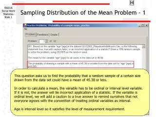
Sampling Distribution of the Sample Mean. Example. Take random sample of 1 hour periods in an ER. Ask “how many patients arrived in that one hour period ?” Calculate statistic, say, the sample mean. Sample 1: 2 3 1 Mean = 2.0 Sample 2: 3 4 2 Mean = 3.0. Situation.

Sampling Distribution of the Sample Mean
E N D
Presentation Transcript
Example • Take random sample of 1 hour periods in an ER. • Ask “how many patients arrived in that one hour period ?” • Calculate statistic, say, the sample mean. Sample 1: 2 3 1 Mean = 2.0 Sample 2: 3 4 2 Mean = 3.0
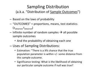
Situation • Different samples produce different results. • Value of a statistic, like mean, SD, or proportion, depends on the particular sample obtained. • But some values may be more likely than others. • The probability distribution of a statistic (“sampling distribution”) indicates the likelihood of getting certain values.
Let’s investigate how sample means and standard deviations vary…. (click here for Live Demo) Web link to try it yourself:http://www.ruf.rice.edu/~lane/stat_sim/sampling_dist/
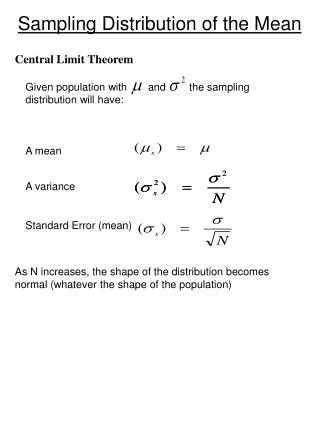
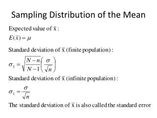
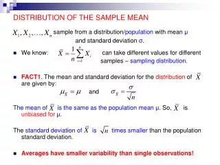
IF: data are normally distributed with mean and standard deviation , and random samples of size n are taken, THEN: The standard deviation of the sample means (“standard error of the mean”) is Sampling Distribution of Sample Mean The sampling distribution of the sample means is also normally distributed. The mean of all of the possible sample means is .
Example • Adult nose length is normally distributed with mean 45 mm and standard deviation 6 mm. • Take random samples of n = 4 adults. • Then, sample means are normally distributed with mean 45 mm and standard error 3 mm[from ].
Using empirical rule... • 68% of samples of n=4 adults will have a sample mean nose length between 42 and 48 mm. • 95% of samples of n=4 adults will have a sample mean nose length between 39 and 51 mm. • 99% of samples of n=4 adults will have a sample mean nose length between 36 and 54 mm.
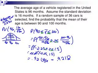
What happens if we take larger samples? • Adult nose length is normally distributed with mean 45 mm and standard deviation 6 mm. • Take random samples of n = 36 adults. • Then, sample means are normally distributed with mean 45 mm and standard error 1 mm [from 6/sqrt(36) = 6/6].
Again, using empirical rule... • 68% of samples of n=36 adults will have a sample mean nose length between 44 and 46 mm. • 95% of samples of n=36 adults will have a sample mean nose length between 43 and 47 mm. • 99% of samples of n=36 adults will have a sample mean nose length between 42 and 48 mm. • So … the larger the sample, the less the sample means vary.
What happens if data are not normally distributed? Let’s investigate that, too …Sampling Distribution Demo: (Live Demo) http://www.ruf.rice.edu/~lane/stat_sim/sampling_dist/
Central Limit Theorem • Even if data are not normally distributed, as long as you take “large enough” samples, the sample averages will at least be approximately normally distributed. • Mean of sample averages is still • Standard error of sample averages is still • In general, “large enough” means more than 30 measurements, but it depends on how non-normal population is to begin with.
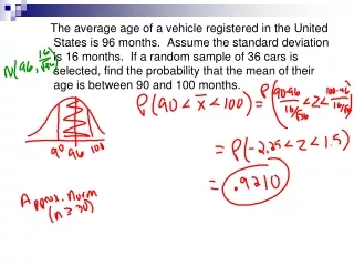
4 3 5 2 4 2 3 1 1 3 0 0 . 6 0 . 8 0 . 0 0 . 2 0 . 4 1 . 0 0 2 2 2 0 . 0 0 . 2 0 . 4 0 . 6 0 . 8 1 . 0 n = 10 1 n = 4 n = 2 n = 1 1 1 0 0 0 . 2 0 . 4 0 . 6 0 . 8 1 . 0 0 0 . 0 0 . 0 0 . 2 0 . 4 0 . 6 0 . 8 1 . 0 0 . 0 0 . 2 0 . 4 0 . 6 0 . 8 1 . 0 The Shape of the Sampling Distribution Population: Triangular X
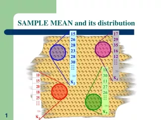
X 2 3 2 2 1 1 1 0 0 0 0 . 0 0 . 2 0 . 4 0 . 6 0 . 8 1 . 0 0 . 0 0 . 2 0 . 4 0 . 6 0 . 8 1 . 0 0 . 4 0 . 0 0 . 2 0 . 6 0 . 8 1 . 0 n = 2 n = 4 n = 10 n = 1 4 3 3 2 2 1 1 0 0 0 . 0 0 . 2 0 . 4 0 . 6 0 . 8 1 . 0 1 . 0 0 . 0 0 . 2 0 . 4 0 . 6 0 . 8 The Shape of the Sampling Distribution Population: Uniform
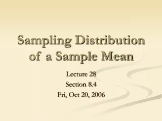
1 . 0 1 . 0 0 . 8 0 . 8 0 . 8 X 0 . 6 0 . 6 0 . 4 0 . 4 0 . 6 0 . 2 0 . 2 0 . 0 0 1 2 3 4 5 6 0 . 0 0 1 2 3 4 5 6 0 . 4 n = 10 n = 4 n = 1 n = 2 0 . 2 1 . 0 1 . 2 0 . 0 0 . 8 0 . 6 0 0 . 8 1 2 3 4 0 . 4 0 . 4 0 . 2 0 . 0 0 . 0 0 1 2 0 1 2 3 The Shape of the Sampling Distribution Population: Exponential
X 3 3 3 2 2 2 1 1 1 0 0 0 0 . 0 0 . 2 0 . 4 0 . 6 0 . 8 1 . 0 0 . 0 0 . 4 0 . 6 0 . 2 0 . 8 1 . 0 0 . 0 0 . 2 0 . 4 0 . 6 0 . 8 1 . 0 n = 2 n = 10 n = 4 n = 1 3 3 2 2 1 1 0 0 0 . 2 0 . 4 0 . 0 0 . 6 0 . 8 1 . 0 0 . 0 0 . 2 0 . 4 0 . 6 0 . 8 1 . 0 The Shape of the Sampling Distribution Population: U-shaped
The Shape of the Sampling Distribution __ (Central Limit Theorem) X is approximatelyNormally distributed for large samples. (i.e. when the sample size n is large)
Big Deal? Let’s look at some useful applications...