Measures of Central Tendency in Statistics
350 likes | 410 Vues
Learn about arithmetic mean, median, mode, and measures of central location in both ungrouped and grouped data sets. Explore how to calculate sample mean, population mean, and properties of mean. Understand the significance of median and mode in data analysis.

Measures of Central Tendency in Statistics
E N D
Presentation Transcript
LESSON 3: CENTRAL TENDENCY Outline • Arithmetic mean, median and mode • Ungrouped data • Grouped data • Percentiles, fractiles, and quartiles • Ungrouped data • Grouped data
MEASURES OF CENTRAL LOCATIONMEAN • Mean is defined as follows: Sum of the measurements Mean = Number of measurements • In the following, sample mean and population means are discussed separately. • Note the difference of notation - sample mean is denote by and the population mean is denoted by . The number of values in a sample is denoted by n and the number of values in the population is denoted by N.
Mean of Data Set Data Set is Data Set is Sample Population Sample Population Mean Mean MEASURES OF CENTRAL LOCATIONMEAN
MEASURES OF CENTRAL LOCATIONSAMPLE MEAN • The sample mean is the sum of all the sample values divided by the number of sample values: • where stands for the sample mean • n is the total number of values in the sample • is the value of the i-th observation • represents a summation
MEASURES OF CENTRAL LOCATIONSAMPLE MEAN • Statistic: a measurable characteristic of a sample. • A sample of five executives received the following amounts of bonus last year: $12,000, $14,000, $18,000, $17,000, and $19,000. Find the average bonus for these five executives. • Since these values represent a sample size of 5, the sample mean is (12,000 + 14,000 +18,000 + 17,000 +19,000)/5 =
MEASURES OF CENTRAL LOCATIONSAMPLE MEAN • Sample mean approximated from grouped data: • Where is the sample mean • is the frequency of the th class interval • is the midpoint of the th class interval • is the total number of observations, • represents a summation
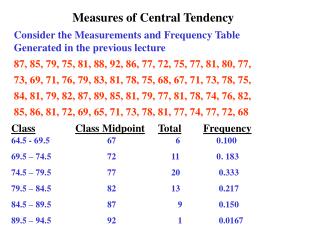
MEASURES OF CENTRAL LOCATIONSAMPLE MEAN • Compute the average days to maturity of 40 investments from the following frequency distribution:
MEASURES OF CENTRAL LOCATIONPOPULATION MEAN • The population mean is the sum of all the population values divided by the number of population values: • Where stands for the population mean • N is the total number of values in the population • is the value of the i-th observation • represents a summation
MEASURES OF CENTRAL LOCATIONPOPULATION MEAN • Parameter: a measurable characteristic of a population. • The Keller family owns four cars. The following is the mileage attained by each car: 55,000, 25,000, 40,000, and 80,000. Find the average miles covered by each car. • The mean is (55,000 + 25,000 + 40,000 + 80,000)/4 =
MEASURES OF CENTRAL LOCATIONPROPERTIES OF MEAN • Data possessing an interval scale or a ratio scale, usually have a mean. • All the values are included in computing the mean. • A set of data has a unique mean. • The mean is affected by unusually large or small data values. • The arithmetic mean is the only measure of central tendency where the sum of the deviations of each value from the mean is zero.
MEASURES OF CENTRAL LOCATIONPROPERTIES OF MEAN • Consider the set of values: 3, 8, and 4. The mean is 5. Illustrating the fifth property, (3-5) + (8-5) + (4-5) = -2 +3 -1 = 0. In other words,
MEASURES OF CENTRAL LOCATIONMEDIAN • Median: The midpoint of the values after they have been ordered from the smallest to the largest, or the largest to the smallest. • There are as many values above the median as below it in the data array. • For an even set of numbers, the median will be the arithmetic average of the two middle numbers. • Median is denoted by
MEASURES OF CENTRAL LOCATIONMEDIAN • After data are ordered • If is odd median is the number • If is even median is the arithmetic average of and number
MEASURES OF CENTRAL LOCATIONMEDIAN • The median is the most appropriate measure of central location to use when the data under consideration are ranked data, rather than quantitative data. • For example, if 13 universities are ranked according to the reputation, university 7 is the one of median reputation.
MEASURES OF CENTRAL LOCATIONMEDIAN • Median is used when few extreme values influence mean too much. For example, one rich family may affect the mean income. So, median income is often reported in place of mean income. • Median is used when all values are not available. For example, in life testing the experiment may end before generating all values. So, mean may not be calculated and median is used instead.
MEASURES OF CENTRAL LOCATIONMEDIAN • Compute the median for the following data. • The age of a sample of five college students is: 21, 25, 19, 20, and 22. • Arranging the data in ascending order gives: • Thus the median is
MEASURES OF CENTRAL LOCATIONMEDIAN • Compute the median for the following data. • The height of four basketball players, in inches, is 76, 73, 80, and 75. • Arranging the data in ascending order gives: • Thus the median is
MEASURES OF CENTRAL LOCATIONMODE • The mode is the value of the observation that appears most frequently. • The mode is most useful when an important aspect of describing the data involves determining the number of times each value occurs. If the data are qualitative (e.g., number of graduate in mechanical, automotive, industrial, etc.) then, mode is useful (e.g., a modal class is mechanical). • For grouped data, mode is the midpoint of the class interval of the highest frequency.
MEASURES OF CENTRAL LOCATIONMODE • EXAMPLE: The exam scores for ten students are: 81, 93, 84, 75, 68, 87, 81, 75, 81, 87. • The modal score =
MEASURES OF CENTRAL LOCATIONMODE • Find the mode for the following grouped data on days to maturity of 40 investments
MEASURES OF CENTRAL LOCATIONMEAN, MEDIAN, MODE • Mean: affected by unusually large/small data, may be used if the data are quantitative (ratio or interval scale). • Median: most appropriate if the data are ranked (ordinal scale) • Mode: most appropriate if the data are qualitative (nominal scale) • Appropriate measures if the data has • ratio or interval scale: mean, median, mode • ordinal scale: median, mode • nominal scale: mode
FINDING MEDIAN AND MODE FROM AN ORDERED STEM-AND-LEAF PLOT Find the median and mode from the following ordered stem-and-leaf plot on days to maturity of 40 investments Stem Leaves 3 1 8 9 4 7 5 0 1 1 3 5 5 6 7 6 0 2 3 4 4 5 6 7 8 9 7 0 0 0 1 5 8 9 8 0 1 3 5 6 7 9 9 5 8 9 9
MEASURES OF CENTRAL LOCATION RELATIVE VALUES OF MEAN, MEDIAN, MODE Mode<Median<Mean If distribution is positively skewed Mode=Median=Mean If distribution is symmetric Mean<Median<Mode if distribution is negatively skewed
RELATIVE STANDINGPERCENTILES, FRACTILES, QUARTILES • Percentiles divide the distribution into 100 groups. • A percentile is a point below which a stated percentage of observations lie. • The p-th percentile is a point below which p% of the values lie. • For example, if the 78th percentile of GMAT scores is 600, then 78% scores are below 600. • Percentiles are not unique. For example, if 78% scores are below 600 and 82% scores are below 610, then the 78th percentile may be any point above 600 and below 610.
RELATIVE STANDINGPERCENTILES, FRACTILES, QUARTILES • Alternate to percentile is fractile. • A fractile is a point below which a stated fraction of observations lie. • The d fractile, is a point below which 100d% of the values lie. • For example, if the 0.78 fractile of GMAT scores is 600, then 78% scores are below 600. Alternate to the 78th percentile is 0.78 fractile. In this case,
RELATIVE STANDINGPERCENTILES, FRACTILES, QUARTILES • Quartiles divide data into four groups of equal frequency. • First quartile = 25th percentile = 0.25 fractile = • Second quartile = 50th percentile = 0.50 fractile = = median • Third quartile = 75th percentile = 0.75 fractile =
RELATIVE STANDING PROCEDURE TO FIND A GIVEN PERCENTILE • Procedure to find . Assume • Step 1: Sort the data in the ascending order (low to high) • Step 2: Find which is the largest integer such that • Step 3: Compute the d fractile i.e., 100d-th percentile as follows • Note: Step 3 finds the required percentile by interpolating between and
RELATIVE STANDING PROCEDURE TO FIND A GIVEN PERCENTILE • Example: Consider data set 2, 3, 5, 6, 8, 10, 12, 15, 18, 20. • Find the 20th percentile • Note: the data set is already ordered. So, Step 1 is not necessary. • Step 2: Find the largest integer So, • Step 3: Compute
RELATIVE STANDING PROCEDURE TO FIND A GIVEN PERCENTILE • Example: Consider data set 2, 3, 5, 6, 8, 10, 12, 15, 18, 20. • Find the 75th percentile • Note: the data set is already ordered. So, Step 1 is not necessary. • Step 2: Find the largest integer So, • Step 3: Compute
RELATIVE STANDING PROCEDURE TO FIND A GIVEN PERCENTILE Find the 80th percentile from the following ordered stem-and-leaf plot on days to maturity of 40 investments Stem Leaves 3 1 8 9 4 7 5 0 1 1 3 5 5 6 7 6 0 2 3 4 4 5 6 7 8 9 7 0 0 0 1 5 8 9 8 0 1 3 5 6 7 9 9 5 8 9 9
RELATIVE STANDING: GROUPED DATA PROCEDURE TO FIND A GIVEN PERCENTILE • For the grouped data, read the percentiles directly from the graph for the cumulative relative frequency distribution. • Find the 80th percentile from the graph for the cumulative relative frequency distribution shown on the next slide and constructed from the data on days to maturity of 40 investments.
OGIVE CUMULATIVE RELATIVE FREQUENCY GRAPH 1.000 1.000 0.900 0.800 0.725 0.600 0.550 Cumulative Frequency 0.400 0.300 0.200 0.100 0.075 0.000 40 50 60 70 80 90 100 Number of Days to Maturity
READING AND EXERCISES Lesson 3 Reading: Section 2-2, pp. 38-47 Exercises: 2-18, 2-20 (and 2-4a), 2-26