Download
1 / 52
520 likes | 713 Vues
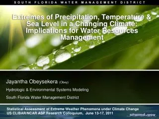
Extremes of Precipitation, Temperature & Sea Level in a Changing Climate: Implications for Water Resources Management . Jayantha Obeysekera (Obey) Hydrologic & Environmental Systems Modeling South Florida Water Management District.

E N D
Extremes of Precipitation, Temperature & Sea Level in a Changing Climate: Implications for Water Resources Management Jayantha Obeysekera (Obey) Hydrologic & Environmental Systems Modeling South Florida Water Management District Statistical Assessment of Extreme Weather Phenomena under Climate Change US CLIBAR/NCAR ASP Research Colloquium, June 13-17, 2011
Outline • Why extremes are important (with emphasis on Florida) – Vulnerabilities in Water Resources Management • A systematic approach to analyze future extremes from models • Historical trends • Validation of models • Conclusions Credit: R-Project, ExtRemes, Fields, RNetCDF packages
Natural Variability – Role of Teleconnections (Kwon, Lall, and Obeysekera (2008)) AMO ENSO Lake Inflow Lake Okeechobee Inflow
A high level conceptual model Climate Change Drivers Water Management Impacts Natural Cycles Interannual (e.g. El Nino and La Nina) to Multi-decadal (e.g. AMO*) Quartet of change: Stressors • Direct landscape impacts (e.g. storm surge) • Water Supply • (e.g. droughts, saltwater intrusion) • Flood Control • (e.g. urban flooding, hurricanes) • Natural Systems • (e.g. ecosystem impacts, both coastal and interior) • Rising Seas • Temperature • Rainfall, floods, and droughts • Tropical Storms & Hurricanes Human Induced Land use changes Greenhouse gases ->Global Warming *Atlantic Multi-decadal Oscillation of temperature in the Atlantic Ocean
Adapatation • Two Important Questions: • Which decisions are likely to be affected and could benefit from adaptation strategies (Type I) in the short term? • “No Regret Strategies” • Which decisions are likely to be affected but for which adaptation strategies (Type II) could be deferred without serious consequences?
Tropical Storms: Natural Variability versus Anthropogenic Effects? Assets Natural Variability? Courtesy: Chris Lansea. National Hurricane Center
Lake Okeechobee Everglades Agricultural Area Water Conservation Areas Lower East Coast Urbanized Area Everglades National Park Pre-Drainage System (1850’s) Managed System (~2003)
Aquifer Storage and Recovery Surface Water Storage Reservoir Stormwater Treatment Areas Seepage Management Removing Barriers to Sheetflow Operational Changes Wastewater Reuse Everglades Restoration
Coastal street flooding during high tide Credit:Joseph Park (SFWMD) Ocean Avenue, A1A Credit: Victoria Morrow (Broward County) Miami-Dade County Credit: Miami-Dade DERM
Impacts of Rising Seas: Flood Control Coastal Structure Ocean Side (tailwater) Land Side(headwater)
Impacts of Rising Seas: Flood Control Coastal Structure Ocean Side (tailwater) Land Side(headwater)
Vulnerable Structures • Preliminary review based on original designs • 28 gravity structures on the East Coast • Six gravity structures on the west coast, including a USACE structure, S-79. • Most vulnerable structures are in Miami Dade and Broward counties
Adaptation to Rising SeasExample: Forward Pumping at S-26 Structure Spillway New Pump Station
Potential Impact of Rising Seas:Southern Everglades • Relocation and possible reduction of mangrove forests • Forced migration of wading birds northward • Potential peat collapse, coastal erosion, and redistribution of sediments • Salinity intrusion into freshwater marshes can: discharge toxic hydrogen sulfide, cause coastal fish kills, and increase habitat loss
50-year rainfall return level- How will these change? 1-hour 6 -hour 12-hour 24-hour 72-hour 120-hour
Resolution (lack of!) GCMs Uncertainties in GCM predictions due to: • Poor resolution – South Florida not even modeled in some GCMs; greater errors at smaller scales • From IPCC AR4-WG1, Ch. 8 - Simulation of tropical precipitation, ENSO, clouds and their response to climate change, etc.
A systematic approach for using climate model data General Ciculation Models (AOGCMs) Observed Climate Data Simulation of Late 20th Century 21st Century Climate Projections Downscale global information to regional information Is there evidence that extremes are changing? How well are climatic extremes represented by GCM/downscaled model results? Role of Teleconnections? How do projections of extremes affect water resources management? 1 2 3
Extreme Value Data Florida, Daily 32 stations Precip, Temp. University of Central Florida, Extreme Values 1 hrs – 120 hrs 68 stations NARCCAP Data Set, 3-hourly, Precip,Temp
Table 1 Statistics used for trend detection Variables Precip Tmax Tmin Tave DTR
May Precipitation May Precipitation - POR (a) May Precipitation – post-1950 (b) 10 0 7 0 Markers sized from +/- 0.2 to +/- 7.7 mm/decade. Markers sized from +/- 0.5 to +/- 21.1 mm/decade.
Number of Dog Days Annual # of Dog Days - POR (a) (b) Annual # of Dog Days – 1950-2008 4 8 3 10 • Markers sized from +/- 0.0 to +/- 6.9 days /decade. • Markers sized from +/- 0.0 to +/- 11.5 days /decade.
Effect of Land Use Changes? Ft. Myers (83186) Trends in annual average daily temperature range (DTR) at (a) Arcadia, (b) Fort Myers, and (c) Fort Lauderdale for the period 1950-2008. The dotted line represents the linear trend from Sen-Theil regression with Zhang’s pre-whitening, while the solid line is the Lowess non-parametric regression line smoother which uses locally-weighted polynomial regression with a span of 0.25. Decadal population estimates for three USHCN stations in Florida. Population estimates were derived by Owen & Gallo (2000) for a 21 km by 21 km grid cell around each station. Arcadia (80228) Ft. Lauderdale (83186) • Historical decrease in the daily temperature range (DTR) for the period 1950-2008 is observed mainly due to increased daily minimum temperature (Tmin) and possibly attributable to heat island effect.
Florida - Main Observations • number of wet days during the dry season – POR • May precipitation throughout the state – POR and especially post-1950. May be linked to changes in start of the wet season. • Urban heat island effect – urban (and drained) areas • Tave and number of dog days for wet (warm) season especially post-1950 • Decrease in DTR ( Tmin > Tmax) • Annual maximum of Tave and Tmin for all seasons in POR and especially post-1950 Hydrologic & Environmental Systems Modeling
A systematic approach for extremes General Ciculation Models (AOGCMs) Observed Climate Data Simulation of Late 20th Century 21st Century Climate Projections Downscale global information to regional information Is there evidence that extremes are changing? How well are climatic extremes represented by GCM/downscaled model results? Role of Teleconnections? How do projections of extremes affect water resources management? 1 2 3
Dynamical DownscalingNorth American Regional Climate Change Assessment Program • Acknowledgement: • NARCCAP is funded by the National Science Foundation (NSF), the U.S. Department of Energy (DoE), the National Oceanic and Atmospheric Administration (NOAA), and the U.S. Environmental Protection Agency Office of Research and Development (EPA)."
NARCCAP Scenario & Models A2 Emissions Scenario GFDL CGCM3 HADCM3 link to European Prudence CCSM CAM3 Time slice 50km GFDL Time slice 50 km Provide boundary conditions 2040-2070 future 1971-2000 current CRCM Quebec, Ouranos RegCM3 UC Santa Cruz ICTP HADRM3 Hadley Centre RSM Scripps WRF NCAR/ PNNL MM5 Iowa State/ PNNL
GEV parameters of annual maxima Scale Shape Location Duration = 6-hours Duration = 24 hours
All locations – Location Parameter 24-Hour 6-Hour
Non-stationarity: Likelihood Ratio Test with AMO as the co-variate on Location Probability Probability 6-hour duration 24-hour duration
Return Level: Current versus Future Current Future Future Current Rainfall (25 year-24 hour) Temperature (50 year-30 day)
Future Projections: Considerable Spread 79 • Resilience • Adaptive Capcity • “no regret strategies” • Adaptive Management • Alternative Futures • Contingency Plans UNEP (2009) Broward 31.5 20 5
Future Projections of Sea Level Rise: Polar Ice Uncertainty Antarctica (~5.4 million sq. km.) Greenland (~ 2 million sq.km.)
What is the future rate of acceleration? Rapid acceleration due to ice sheet loss Sea Level Rise relative to 2010 (mm) Medium acceleration Continuing current trend
Probability Distribution of Extremes Total Sea Level Rise , • T(t) = G(t) + L(t) • Global Local • G(t) = b t + 0.5a t2 • T(t) = [L(t) + b t] + 0.5a t2 • = c t + 0.5a t2
Probability Distribution of Extremes Assume Annual Maxima of SLR ~ Generalize Extreme Value (GEV) Distribution TE,t ~ GEV(μt , , ) and location, μ t = T(t)+ e p-year return level: e
Summary • Water Resource Management in South Florida is highly vulnerable to potential changes in both climate and sea level rise • Skills of regional climate models in predicting extremes may not be adequate for decision making. • Water managers need methods to deal with uncertainties in decision making
Questions! Recent cabinet meeting of the island nation, Maldives