Electromagnetic Waves and Transmission Line Principles in Lecture 3 of 16.360
170 likes | 290 Vues
This lecture delves into the principles of electromagnetic waves and transmission lines, focusing on concepts such as magnetic fields produced by constant currents, traveling wave equations, phasor representations, and their applications in solving integral and differential equations. Key topics include the relationship between frequency, wavelength, and wave propagation, transmission line parameters, input impedance, and power flow. The session also discusses fiber optics, effective communication wavelengths, and concludes with insights on types of transmission lines and the lumped-element model.

Electromagnetic Waves and Transmission Line Principles in Lecture 3 of 16.360
E N D
Presentation Transcript
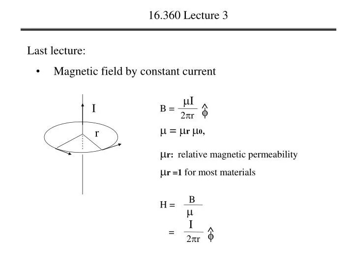
I I r B = 2r B H = I = 2r 16.360 Lecture 3 Last lecture: • Magnetic field by constant current = r 0, r: relative magnetic permeability r =1 for most materials
16.360 Lecture 3 Last lecture: • Traveling wave y(x,t) = Acos(2t/T-2x/), y(x,t) = Acos(x,t), (x,t) = 2t/T-2x/,
16.360 Lecture 3 Last lecture: • Traveling wave y(x,t) = Acos(2t/T+2x/), Velocity = 0.6/0.6T = /T Phase velocity: Vp = dx/dt = - /T
Vs(t) VC(t) i (t) i(t)dt/C, VC(t) = 16.360 Lecture 3 • Phasor VR(t) Vs(t) = V0Sin(t+0), VR(t) = i(t)R, Vs(t) = VR(t) +VC(t), V0Sin(t+0) = i(t)dt/C + i(t)R, Integral equation, Using phasor to solve integral and differential equations
jt ) Z(t) = Re( Z e Z is time independent function of Z(t), i.e. phasor jt jt e e = Re(V ), j(0 - /2) , V = V0 e 16.360 Lecture 3 • Phasor Vs(t) = V0Sin(t+0) j(0 - /2) ) = Re(V0 e
jt ) i(t) = Re( I e 1 jt )/C + = Re(I i(t)dt= Re( I e )dt j jt jt jt e e e jt ), Re( I e Re(V ) 16.360 Lecture 3 • Phasor 1 ), = Re(I j time domain equation: V0Sin(t+0) = i(t)dt/C + i(t)R, phasor domain equation:
jt 1 = I ) i(t) = Re( I e jC V j(0 - /2) j(0 - /2) V0 e V0 e 16.360 Lecture 3 • Phasor domain V + I R , I = R + 1/(jC) = , R + 1/(jC) Back to time domain: jt e = Re ( ) R + 1/(jC)
16.360 Lecture 3 • An Example : VR(t) Vs(t) = V0Sin(t+0), VR(t) = i(t)R, Vs(t) VL(t) i (t) Ldi(t)/dt, VL(t) = Vs(t) = VR(t) +VL(t), V0Sin(t+0) = Ldi(t)/dt + i(t)R, differential equation, Using phasor to solve the differential equation.
jt ) i(t) = Re( I e jt jt jt e e e jt ), Re( I e Re(V ) 16.360 Lecture 3 • Phasor jt di(t)/dt= Re(d I e )/dt j = Re(I ), time domain equation: V0Sin(t+0) = Ldi(t)/dt + i(t)R, phasor domain equation: j )L + = Re(I
jt ) i(t) = Re( I e V j(0 - /2) j(0 - /2) V0 e V0 e 16.360 Lecture 3 • Phasor domain jL + I R V = I , I = R + (jL) = , R + jL) Back to time domain: jt e = Re ( ) R + (jL)
16.360 Lecture 3 • Steps of transferring integral or differential equations to linear • equations using phasor. • Express time-dependent variables as phsaor. • Rewrite integral or differential equations in phasor domain. • Solve phasor domain equations • Change phasors variable to their time domain value
16.360 Lecture 3 • Electromagnetic spectrum. Recall relation: f = v. • Some important wavelength ranges: • Fiber optical communication: = 1.3 – 1.5m. • Free space communication: ~ 700nm – 980nm. • TV broadcasting and cellular phone: 300MHz – 3GHz. • Radar and remote sensing: 30GHz – 300GHz
16.360 Lecture 3 • Transmission lines • Transmission line parameters, equations • Wave propagations • Lossless line, standing wave and reflection coefficient • Input impedence • Special cases of lossless line • Power flow • Smith chart • Impedence matching • Transients on transmission lines
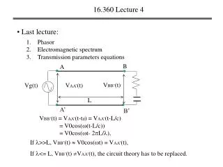
16.360 Lecture 3 • Today • Transmission line parameters, equations B A VBB’(t) Vg(t) VAA’(t) L A’ B’ VAA’(t) = Vg(t) = V0cos(t), Low frequency circuits: VBB’(t) = VAA’(t) Approximate result VBB’(t) = VAA’(t-td) = VAA’(t-L/c) = V0cos((t-L/c)),
B A VBB’(t) Vg(t) VAA’(t) L A’ B’ 16.360 Lecture 3 • Transmission line parameters, equations Recall: =c, and = 2 VBB’(t) = VAA’(t-td) = VAA’(t-L/c) = V0cos((t-L/c)) = V0cos(t- 2L/), If >>L, VBB’(t) V0cos(t) = VAA’(t), If <= L, VBB’(t) VAA’(t), the circuit theory has to be replaced.
16.360 Lecture 3 • Next lecture • Types of transmission lines • Lumped-element model • Transmission line equations • Wave propagation