Understanding Transmission Line Parameters and Equations in Electromagnetics
This lecture focuses on transmission line parameters, essential equations, and their applications in electromagnetic theory. It covers key topics such as phasor representations, types of transmission lines (including coaxial, two-wire, optical fiber, and waveguides), and fundamental equations like the Telegrapher’s equations. We explore the lumped-element model and discuss critical concepts like time delay, reflection, power loss, and dispersion. Understanding these principles is crucial for analyzing signal propagation in various transmission media.

Understanding Transmission Line Parameters and Equations in Electromagnetics
E N D
Presentation Transcript
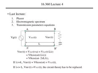
B A VBB’(t) Vg(t) VAA’(t) L A’ B’ 16.360 Lecture 4 • Last lecture: • Phasor • Electromagnetic spectrum • Transmission parameters equations VBB’(t) = VAA’(t-td) = VAA’(t-L/c) = V0cos((t-L/c)) = V0cos(t- 2L/), If >>L, VBB’(t) V0cos(t) = VAA’(t), If <= L, VBB’(t) VAA’(t), the circuit theory has to be replaced.
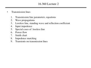
16.360 Lecture 4 • Today: • Transmission line parameters • Types of transmission lines • Lumped-element model • Transmission line equations • Telegrapher’s equations • Wave equations
B A VBB’(t) Vg(t) VAA’(t) L A’ B’ 16.360 Lecture 4 • Transmission line parameters • time delay VBB’(t) = VAA’(t-td) = VAA’(t-L/vp), • Reflection: the voltage has to be treat as wave, some bounce back • power loss: due to reflection and some other loss mechanism, • Dispersion: in material, Vp could be different for different wavelength
B E 16.360 Lecture 4 • Types of transmission lines • Transverse electromagnetic (TEM) transmission lines B E a) Coaxial line b) Two-wire line c) Parallel-plate line d) Strip line e) Microstrip line
16.360 Lecture 4 • Types of transmission lines • Higher-order transmission lines a) Optical fiber b) Rectangular waveguide c) Coplanar waveguide
16.360 Lecture 4 • Lumped-element Model • Represent transmission lines as parallel-wire configuration A B Vg(t) VBB’(t) VAA’(t) B’ A’ z z z R’z L’z L’z R’z L’z R’z Vg(t) G’z C’z C’z C’z G’z G’z
16.360 Lecture 4 • Transmission line equations • Represent transmission lines as parallel-wire configuration i(z,t) i(z+z,t) L’z R’z V(z,t) V(z+ z,t) G’z C’z V(z,t) = R’z i(z,t) + L’z i(z,t)/ t + V(z+ z,t), (1) i(z,t) = G’z V(z+ z,t) + C’z V(z+ z,t)/t + i(z+z,t), (2)
i(z,t) i(z+z,t) L’z R’z V(z,t) V(z+ z,t) G’z C’z jt jt V(z,t) = Re( V(z) e i (z,t) = Re( i (z) e ), ), 16.360 Lecture 4 • Transmission line equations V(z,t) = R’z i(z,t) + L’z i(z,t)/ t + V(z+ z,t), (1) -V(z+ z,t) + V(z,t) = R’z i(z,t) + L’z i(z,t)/ t - V(z,t)/z = R’ i(z,t) + L’ i(z,t)/ t, (3) Rewrite V(z,t) and i(z,t) as phasors, for sinusoidal V(z,t) and i(z,t):
i(z,t) i(z+z,t) L’z R’z V(z,t) V(z+ z,t) G’z C’z jt e j = Re(i ), - dV(z)/dz = R’ i(z) + jL’ i(z), (4) 16.360 Lecture 4 • Transmission line equations Recall: jt di(t)/dt= Re(d i e )/dt - V(z,t)/z = R’ i(z,t) + L’ i(z,t)/ t, (3)
16.360 Lecture 4 • Transmission line equations • Represent transmission lines as parallel-wire configuration i(z,t) i(z+z,t) L’z R’z V(z,t) V(z+ z,t) G’z C’z V(z,t) = R’z i(z,t) + L’z i(z,t)/ t + V(z+ z,t), (1) i(z,t) = G’z V(z+ z,t) + C’z V(z+ z,t)/t + i(z+z,t), (2)
i(z,t) i(z+z,t) L’z R’z V(z,t) V(z+ z,t) G’z C’z jt jt V(z,t) = Re( V(z) e i (z,t) = Re( i (z) e ), ), 16.360 Lecture 4 • Transmission line equations i(z,t) = G’z V(z+ z,t) + C’z V(z+ z,t)/t + i(z+z,t), (2) - i (z+ z,t) + i (z,t) = G’z V(z + z ,t) + C’z V(z + z,t)/ t - i(z,t)/z = G’ V(z,t) + C’ V(z,t)/ t, (5) Rewrite V(z,t) and i(z,t) as phasors, for sinusoidal V(z,t) and i(z,t):
i(z,t) i(z+z,t) L’z R’z V(z,t) V(z+ z,t) G’z C’z jt e j = Re(V ), - d i(z)/dz = G’ V(z) + jC’ V(z), (7) 16.360 Lecture 4 • Transmission line equations Recall: jt dV(t)/dt= Re(d V e )/dt - i(z,t)/z = G’ V(z,t) + C’ V(z,t)/ t, (6)
i(z,t) i(z+z,t) L’z R’z V(z,t) V(z+ z,t) G’z C’z - d i(z)/dz = G’ V(z) + jC’ V(z), (7) - dV(z)/dz = R’ i(z) + jL’ i(z), (4) - d²V(z)/dz² = R’ di(z)/dz + jL’ di(z)/dz, (8) 16.360 Lecture 4 • Telegrapher’s equation in phasor domain Take d /dz on both sides of eq. (4)
- dV(z)/dz = R’ i(z) + jL’ i(z), (4) - d²V(z)/dz² = R’ di(z)/dz + jL’ di(z)/dz, (8) 16.360 Lecture 4 • Telegrapher’s equation in phasor domain - d i(z)/dz = G’ V(z) + jC’ V(z), (7) substitute (7) to (8) d²V(z)/dz² = (R’ + jL’) (G’+ jC’)V(z), or d²V(z)/dz² - (R’ + jL’) (G’+ jC’)V(z) = 0, (9) d²V(z)/dz² - ²V(z) = 0, (10) ² = (R’ + jL’) (G’+ jC’), (11)
i(z,t) i(z+z,t) L’z R’z V(z,t) V(z+ z,t) G’z C’z - d i(z)/dz = G’ V(z) + jC’ V(z), (7) - dV(z)/dz = R’ i(z) + jL’ i(z), (4) 16.360 Lecture 4 • Telegrapher’s equation in phasor domain Take d /dz on both sides of eq. (7) - d² i(z)/dz² = G’ dV(z)/dz + jC’ dV(z)/dz, (12)
- dV(z)/dz = R’ i(z) + jL’ i(z), (4) 16.360 Lecture 4 • Telegrapher’s equation in phasor domain - d i(z)/dz = G’ V(z) + jC’ V(z), (7) - d² i(z)/dz² = G’ dV(z)/dz + jC’ dV(z)/dz, (12) substitute (4) to (12) d² i(z)/dz² = (R’ + jL’) (G’+ jC’)i(z), or d² i(z)/dz² - (R’ + jL’) (G’+ jC’) i(z) = 0, (9) d² i(z)/dz² - ²i(z) = 0, (13) ² = (R’ + jL’) (G’+ jC’), (11)
= Re (R’ + jL’) (G’+ jC’) , = Im (R’ + jL’) (G’+ jC’) , 16.360 Lecture 4 • Wave equations d²V(z)/dz² - ²V(z) = 0, (10) d² i(z)/dz² - ²i(z) = 0, (13) = + j,
16.360 Lecture 4 • Summary • Transmission line parameters • Types of transmission lines • Lumped-element model • Transmission line equations • Telegrapher’s equations • Wave equations
16.360 Lecture 4 • Next lecture • Wave propagation on a Transmission line • Characteristic impedance • Standing wave and traveling wave • Lossless transmission line • Reflection coefficient