Download

1 / 10
100 likes | 287 Vues
16.360 Lecture 4. Transmission lines. Transmission line parameters, equations Wave propagations Lossless line, standing wave and reflection coefficient Input impedence Special cases of lossless line Power flow Smith chart Impedence matching Transients on transmission lines.

E N D
16.360 Lecture 4 • Transmission lines • Transmission line parameters, equations • Wave propagations • Lossless line, standing wave and reflection coefficient • Input impedence • Special cases of lossless line • Power flow • Smith chart • Impedence matching • Transients on transmission lines
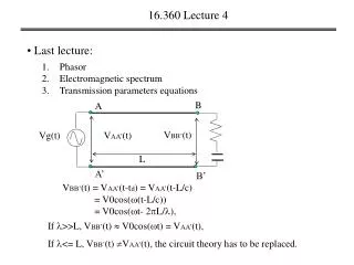
16.360 Lecture 4 • Transmission line parameters, equations B A VBB’(t) = VAA’(t) VBB’(t) Vg(t) VAA’(t) L A’ B’ VAA’(t) = Vg(t) = V0cos(t), Low frequency circuits: VBB’(t) = VAA’(t) Approximate result VBB’(t) = VAA’(t-td) = VAA’(t-L/c) = V0cos((t-L/c)),
B A VBB’(t) Vg(t) VAA’(t) L A’ B’ 16.360 Lecture 4 • Transmission line parameters, equations Recall: =c, and = 2 VBB’(t) = VAA’(t-td) = VAA’(t-L/c) = V0cos((t-L/c)) = V0cos(t- 2L/), If >>L, VBB’(t) V0cos(t) = VAA’(t), If <= L, VBB’(t) VAA’(t), the circuit theory has to be replaced.
B A VBB’(t) Vg(t) VAA’(t) L A’ B’ 16.360 Lecture 4 • Transmission line parameters, equations e. g: = 1GHz, L = 1cm Time delay t = L/c = 1cm /3x1010 cm/s = 30 ps Phase shift = 2ft = 0.06 VBB’(t) = VAA’(t) = 10GHz, L = 1cm Time delay t = L/c = 1cm /3x1010 cm/s = 30 ps Phase shift = 2ft = 0.6 VBB’(t) VAA’(t)
B A VBB’(t) Vg(t) VAA’(t) L A’ B’ 16.360 Lecture 4 • Transmission line parameters • time delay VBB’(t) = VAA’(t-td) = VAA’(t-L/vp), • Reflection: the voltage has to be treat as wave, some bounce back • power loss: due to reflection and some other loss mechanism, • Dispersion: in material, Vp could be different for different wavelength
B E 16.360 Lecture 4 • Types of transmission lines • Transverse electromagnetic (TEM) transmission lines B E a) Coaxial line b) Two-wire line c) Parallel-plate line d) Strip line e) Microstrip line
16.360 Lecture 4 • Types of transmission lines • Higher-order transmission lines a) Optical fiber b) Rectangular waveguide c) Coplanar waveguide
16.360 Lecture 4 • Lumped-element Model • Represent transmission lines as parallel-wire configuration A B Vg(t) VBB’(t) VAA’(t) B’ A’ z z z R’z L’z L’z R’z L’z R’z Vg(t) G’z C’z C’z C’z G’z G’z
Definitions of TL dimensions TEM (Transverse Electromagnetic): Electric and magnetic fields are orthogonal to one another, and both are orthogonal to direction of propagation