Understanding Short Circuit and Open Circuit Lines in Transmission Line Theory
This lecture focuses on the principles of short circuit and open circuit lines in transmission line theory. It explores important concepts like quarter-wave transformers and matched transmission lines, highlighting their significance in power transmission. The mathematical analysis includes expressions for input impedance, power flow, and the various conditions under which transmission lines behave as capacitive or inductive. Additionally, the application of network analyzers for measuring S-parameters and calculating characteristic impedance is discussed.

Understanding Short Circuit and Open Circuit Lines in Transmission Line Theory
E N D
Presentation Transcript
16.360 Lecture 8 • Last lecture • short circuit line • open circuit line • quarter-wave transformer • matched transmission line
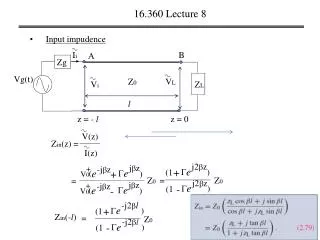
+ V0 Z0 jz jz -jz -jz e (e e (e 16.360 Lecture 8 short circuit line B Ii A Zg Vg(t) sc Z0 VL Zin ZL = 0 l z = - l z = 0 ZL= 0, = -1, S = + V(z) = V0 ) - = -2jV0sin(z) + + i(z) = ) = 2V0cos(z)/Z0 V(-l) Zin = jZ0tan(l) = i(-l)
-1 l = 1/[- tan (1/CeqZ0)], 16.360 Lecture 8 short circuit line V(-l) Zin = jZ0tan(l) = i(-l) • If tan(l) >= 0, the line appears inductive, jLeq= jZ0tan(l), • If tan(l) <= 0, the line appears capacitive, 1/jCeq= jZ0tan(l), • The minimum length results in transmission line as a capacitor:
+ = 2V0cos(z) + V0 Z0 jz jz -jz -jz e (e e (e 16.360 Lecture 8 open circuit line B Ii A Zg Vg(t) oc Z0 VL Zin ZL = l z = - l z = 0 ZL= 0, = 1, S = + V(z) = V0 ) + - i(z) = ) = 2jV0sin(z)/Z0 V(-l) oc Zin = -jZ0cot(l) = i(-l)
oc sc Zin Zin • Measure and sc oc = -jZ0cot(l) = jZ0tan(l) Zin Zin oc sc sc oc Zin Zin Zin Zin Z0 = Z0 = -j 16.360 Lecture 8 Application for short-circuit and open-circuit • Network analyzer • Measure S paremeters • Calculate Z0 • Calculate l
-j2l -j2l e e + - (1 (1 ) ) Z0 16.360 Lecture 8 Transmission line of length l = n/2 tan(l) = tan((2/)(n/2)) = 0, Zin(-l) = = ZL Any multiple of half-wavelength line doesn’t modify the load impedance.
(1 - ) Z0 (1 + ) -j2l -j2l e e - + (1 (1 ) ) Z0 16.360 Lecture 8 Quarter-wave transformer l = /4 + n/2 l = (2/)(/4 + n/2) = /2 , -j e + ) (1 Zin(-l) = = Z0 = -j e - (1 ) = Z0²/ZL
16.360 Lecture 8 Matched transmission line: • ZL = Z0 • = 0 • All incident power is delivered to the load.
- + + V0 V0 V0 Z0 Z0 Z0 -jz jz -jz e e (e 16.360 Lecture 8 Today: Power flow on a lossless transmission line • Instantaneous power • Time-average power jz + e V(z) = V0() + - i(z) = ) At load z = 0, the incident and reflected voltages and currents: i i + V = V0 i = r - r V = V0 i =
16.360 Lecture 8 • Instantaneous power i i i P(t) = v(t) i(t) = Re[V exp(jt)] Re[ i exp(jt)] + + + + = Re[|V0|exp(j )exp(jt)] Re[|V0|/Z0 exp(j )exp(jt)] + + = (|V0|²/Z0) cos²(t + ) r r r P(t) = v(t) i(t) = Re[V exp(jt)] Re[ i exp(jt)] - + - + = Re[|V0|exp(j )exp(jt)] Re[|V0|/Z0 exp(j )exp(jt)] + + = - ||²(|V0|²/Z0) cos²(t + + r)
1 T + + (|V0|²/Z0) cos²(t + )dt 16.360 Lecture 8 • Time-average Time-domain approach: i T T i Pav = P (t)dt = 2 0 0 + = (|V0|²/2Z0) r + Pav = -||² (|V0|²/2Z0) Net average power: i r Pav + Pav = Pav + = (1-||²) (|V0|²/2Z0)
16.360 Lecture 8 • Time-average Phasor-domain approach Pav = (½)Re[V i*] i + + Pav = (1/2) Re[V0 V0*/Z0] = (|V0|²/2Z0) r + Pav = -||² (|V0|²/2Z0) + Pav = (1-||²) (|V0|²/2Z0)
16.360 Lecture 8 Next lecture • The Smith Chart