Analyzing First Order Decay Equations in Graphical Data Analysis
This document explores the principles of first-order decay through mathematical equations and graphical data analysis. It discusses the rate of change of concentration over time, provided by the differential equation d[A]/dt = -k[A], and its integration to yield the exponential decay function. The concept of equilibrium is also introduced, emphasizing observable data relationships such as molar concentration and fraction of total presence. Key algebraic manipulations are presented, demonstrating how to rearrange and interpret decay equations for effective analysis.

Analyzing First Order Decay Equations in Graphical Data Analysis
E N D
Presentation Transcript
Graphical Data Analysis CHM 2051 Computer Homework 2.5
First Order Decay - Equations • Rate = d[A]/dt = - k [A] • [A] = [A]0 exp( - k t) (exponential decay) • ln [A] = ln [A]0 - k t slope = k intercept = ln [A] 0
Equilibrium Data E + X EX [EX] K = -------------- [E] [X]
Observable Data • [X] (molar concentration of X) [EX] • Y = ----------------- ([E] + [EX]) (fraction of total E present as EX)
Functional Form of Y Variable K [X] • Y = ------------------ (1 + K [X]) • Initial slope = K • Limit at high [X] = 1
Some Simple Algebra K [X] • Y = ------------------ (as before) (1 + K [X]) Rearranges as: Y ( ----------- ) = K [X] 1 - Y slope = K intercept = 0